numpy.random.standard_cauchy#
- random.standard_cauchy(size=None)#
从中心点为 0 的标准 Cauchy 分布中抽取样本。
也称为洛伦兹分布。
注意
新代码应使用
Generator实例的standard_cauchy方法;请参阅 快速入门。- 参数:
- sizeint 或 int 的元组,可选
输出形状。如果给定的形状例如是
(m, n, k),则将抽取m * n * k个样本。默认为 None,在这种情况下返回单个值。
- 返回:
- samplesndarray 或标量
绘制的样本。
另请参阅
random.Generator.standard_cauchy新代码应使用此方法。
备注
完整柯西分布的概率密度函数为
\[P(x; x_0, \gamma) = \frac{1}{\pi \gamma \bigl[ 1+ (\frac{x-x_0}{\gamma})^2 \bigr] }\]而标准柯西分布只是设置 \(x_0=0\) 和 \(\gamma=1\)
柯西分布出现在受迫振动振荡器问题的解中,也描述了光谱线展宽。它还描述了以随机角度倾斜的直线与 x 轴相交的值的分布。
在研究假设检验(假设正态性)时,查看检验在来自柯西分布的数据上的表现,是衡量其对重尾分布敏感度的良好指标,因为柯西分布非常类似于高斯分布,但尾部更重。
参考
[1]NIST/SEMATECH e-Handbook of Statistical Methods,“Cauchy Distribution”,https://www.itl.nist.gov/div898/handbook/eda/section3/eda3663.htm
[2]Weisstein, Eric W. “Cauchy Distribution.” 来自 MathWorld–A Wolfram Web Resource。https://mathworld.net.cn/CauchyDistribution.html
[3]Wikipedia,“Cauchy distribution” https://en.wikipedia.org/wiki/Cauchy_distribution
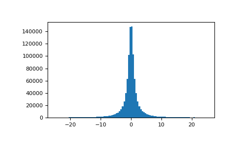
示例
绘制样本并绘制分布图
>>> import matplotlib.pyplot as plt
>>> s = np.random.standard_cauchy(1000000)
>>> s = s[(s>-25) & (s<25)]  # truncate distribution so it plots well
>>> plt.hist(s, bins=100)
>>> plt.show()