numpy.random.Generator.gumbel

方法

random.Generator.gumbel(loc=0.0, scale=1.0, size=None)

从具有指定位置（或均值）和尺度（衰减）的 Gumbel 分布中抽取样本。

从具有指定位置和尺度的 Gumbel 分布中抽取样本。有关 Gumbel 分布的更多信息，请参阅下面的“注”和“参考文献”。

参数:

locfloat 或 array_like of floats, optional

分布模式的位置。默认为 0。

scalefloat 或 array_like of floats, optional

分布的尺度参数。默认为 1。必须为非负数。

sizeint 或 int 的元组，可选

输出形状。如果给定的形状是，例如，(m, n, k)，则绘制 m * n * k 个样本。如果 size 为 None（默认），则当 loc 和 scale 均为标量时，将返回单个值。否则，将绘制 np.broadcast(loc, scale).size 个样本。

返回:

outndarray 或标量

从参数化的 Gumbel 分布中抽取的样本。

另请参阅

scipy.stats.gumbel_l

scipy.stats.gumbel_r

scipy.stats.genextreme

韦布尔

备注

Gumbel 分布（或最小极值（SEV）或最小极值 I 型）是一类广义极值（GEV）分布，用于对极值问题进行建模。Gumbel 分布是指数型尾部分布的最大值极值 I 型分布的一个特例。

Gumbel 分布的概率密度为

\[p(x) = \frac{e^{-(x - \mu)/ \beta}}{\beta} e^{ -e^{-(x - \mu)/ \beta}},\]

其中 \(\mu\) 是模式，一个位置参数，\(\beta\) 是尺度参数。

Gumbel 分布（以德国数学家 Emil Julius Gumbel 的名字命名）很早就被用于水文学文献中，用于模拟洪水事件的发生。它也用于模拟最大风速和降雨率。它是一个“肥尾”分布——尾部事件发生的概率比高斯分布大，因此 100 年一遇的洪水发生频率出人意料地高。洪水最初被建模为高斯过程，这低估了极端事件的频率。

它是极值分布的一类，即广义极值（GEV）分布，其中还包括 Weibull 分布和 Frechet 分布。

该函数具有均值 \(\mu + 0.57721\beta\) 和方差 \(\frac{\pi^2}{6}\beta^2\)。

参考

[1]

Gumbel, E. J., “Statistics of Extremes,” New York: Columbia University Press, 1958。

[2]

Reiss, R.-D. and Thomas, M., “Statistical Analysis of Extreme Values from Insurance, Finance, Hydrology and Other Fields,” Basel: Birkhauser Verlag, 2001。

示例

在浏览器中尝试！

从分布中绘制样本

>>> rng = np.random.default_rng()
>>> mu, beta = 0, 0.1 # location and scale
>>> s = rng.gumbel(mu, beta, 1000)

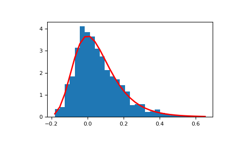
显示样本的直方图以及概率密度函数

>>> import matplotlib.pyplot as plt
>>> count, bins, _ = plt.hist(s, 30, density=True)
>>> plt.plot(bins, (1/beta)*np.exp(-(bins - mu)/beta)
...          * np.exp( -np.exp( -(bins - mu) /beta) ),
...          linewidth=2, color='r')
>>> plt.show()

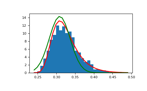
展示极值分布如何从高斯过程产生，并与高斯分布进行比较

>>> means = []
>>> maxima = []
>>> for i in range(0,1000) :
...    a = rng.normal(mu, beta, 1000)
...    means.append(a.mean())
...    maxima.append(a.max())
>>> count, bins, _ = plt.hist(maxima, 30, density=True)
>>> beta = np.std(maxima) * np.sqrt(6) / np.pi
>>> mu = np.mean(maxima) - 0.57721*beta
>>> plt.plot(bins, (1/beta)*np.exp(-(bins - mu)/beta)
...          * np.exp(-np.exp(-(bins - mu)/beta)),
...          linewidth=2, color='r')
>>> plt.plot(bins, 1/(beta * np.sqrt(2 * np.pi))
...          * np.exp(-(bins - mu)**2 / (2 * beta**2)),
...          linewidth=2, color='g')
>>> plt.show()

返回在新标签页中打开