

NumPy 快速入门#
先决条件#
你需要了解一些 Python。如需复习,请参阅 Python 教程。
要运行示例,除了 NumPy,你还需要安装 matplotlib。
学习者概况
这是对 NumPy 中数组的快速概述。它演示了 n 维(\(n>=2\))数组是如何表示和操作的。特别是,如果你不知道如何将常用函数应用于 n 维数组(不使用 for 循环),或者如果你想了解 n 维数组的轴和形状属性,本文可能会有所帮助。
学习目标
阅读后,你应该能够
理解 NumPy 中一维、二维和 n 维数组的区别;
理解如何在不使用 for 循环的情况下将一些线性代数操作应用于 n 维数组;
理解 n 维数组的轴和形状属性。
基础知识#
NumPy 的主要对象是同质多维数组。它是一个元素表(通常是数字),所有元素都具有相同类型,通过非负整数元组进行索引。在 NumPy 中,维度被称为 轴。
例如,三维空间中一个点的坐标数组 [1, 2, 1] 具有一个轴。该轴包含 3 个元素,因此我们说它的长度为 3。在下图所示的示例中,数组具有 2 个轴。第一个轴的长度为 2,第二个轴的长度为 3。
[[1., 0., 0.],
 [0., 1., 2.]]
NumPy 的数组类名为 ndarray。它也以别名 array 著称。请注意,numpy.array 与标准 Python 库中的 array.array 类不同,后者只处理一维数组,功能较少。ndarray 对象更重要的属性是
- ndarray.ndim
数组的轴(维度)数量。
- ndarray.shape
数组的维度。这是一个整数元组,指示数组在每个维度上的大小。对于一个具有 n 行 m 列的矩阵,
shape将是(n,m)。shape元组的长度因此是轴的数量,即ndim。- ndarray.size
数组的元素总数。这等于
shape中元素的乘积。- ndarray.dtype
描述数组中元素类型的对象。可以使用标准 Python 类型创建或指定 dtype。此外,NumPy 提供自己的类型。numpy.int32、numpy.int16 和 numpy.float64 是一些示例。
- ndarray.itemsize
数组中每个元素的字节大小。例如,一个类型为
float64的数组,其itemsize为 8 (=64/8),而类型为complex32的数组,其itemsize为 4 (=32/8)。它等同于ndarray.dtype.itemsize。- ndarray.data
包含数组实际元素的缓冲区。通常,我们不需要使用此属性,因为我们将使用索引工具访问数组中的元素。
一个例子#
>>> import numpy as np
>>> a = np.arange(15).reshape(3, 5)
>>> a
array([[ 0,  1,  2,  3,  4],
       [ 5,  6,  7,  8,  9],
       [10, 11, 12, 13, 14]])
>>> a.shape
(3, 5)
>>> a.ndim
2
>>> a.dtype.name
'int64'
>>> a.itemsize
8
>>> a.size
15
>>> type(a)
<class 'numpy.ndarray'>
>>> b = np.array([6, 7, 8])
>>> b
array([6, 7, 8])
>>> type(b)
<class 'numpy.ndarray'>
数组创建#
有几种创建数组的方法。
例如,您可以使用 array 函数从普通的 Python 列表或元组创建数组。结果数组的类型是根据序列中元素的类型推断出来的。
>>> import numpy as np
>>> a = np.array([2, 3, 4])
>>> a
array([2, 3, 4])
>>> a.dtype
dtype('int64')
>>> b = np.array([1.2, 3.5, 5.1])
>>> b.dtype
dtype('float64')
一个常见的错误是调用 array 时提供多个参数,而不是提供一个单一序列作为参数。
>>> a = np.array(1, 2, 3, 4)    # WRONG
Traceback (most recent call last):
  ...
TypeError: array() takes from 1 to 2 positional arguments but 4 were given
>>> a = np.array([1, 2, 3, 4])  # RIGHT
array 将序列的序列转换为二维数组,将序列的序列的序列转换为三维数组,依此类推。
>>> b = np.array([(1.5, 2, 3), (4, 5, 6)])
>>> b
array([[1.5, 2. , 3. ],
       [4. , 5. , 6. ]])
数组的类型也可以在创建时明确指定
>>> c = np.array([[1, 2], [3, 4]], dtype=complex)
>>> c
array([[1.+0.j, 2.+0.j],
       [3.+0.j, 4.+0.j]])
通常,数组的元素最初是未知的,但其大小是已知的。因此,NumPy 提供了几个函数来创建具有初始占位符内容的数组。这最大限度地减少了数组扩展的必要性,因为扩展数组是一项昂贵的操作。
函数 zeros 创建一个全零数组,函数 ones 创建一个全一数组,而函数 empty 创建一个初始内容是随机的,取决于内存状态的数组。默认情况下,创建的数组的 dtype 是 float64,但可以通过关键字参数 dtype 指定。
>>> np.zeros((3, 4))
array([[0., 0., 0., 0.],
       [0., 0., 0., 0.],
       [0., 0., 0., 0.]])
>>> np.ones((2, 3, 4), dtype=np.int16)
array([[[1, 1, 1, 1],
        [1, 1, 1, 1],
        [1, 1, 1, 1]],

       [[1, 1, 1, 1],
        [1, 1, 1, 1],
        [1, 1, 1, 1]]], dtype=int16)
>>> np.empty((2, 3))
array([[3.73603959e-262, 6.02658058e-154, 6.55490914e-260],  # may vary
       [5.30498948e-313, 3.14673309e-307, 1.00000000e+000]])
为了创建数字序列,NumPy 提供了 arange 函数,它类似于 Python 内置的 range,但返回一个数组。
>>> np.arange(10, 30, 5)
array([10, 15, 20, 25])
>>> np.arange(0, 2, 0.3)  # it accepts float arguments
array([0. , 0.3, 0.6, 0.9, 1.2, 1.5, 1.8])
当 arange 与浮点参数一起使用时,由于浮点精度有限,通常无法预测获得的元素数量。因此,通常最好使用函数 linspace,它将我们想要的元素数量作为参数,而不是步长。
>>> from numpy import pi
>>> np.linspace(0, 2, 9)                   # 9 numbers from 0 to 2
array([0.  , 0.25, 0.5 , 0.75, 1.  , 1.25, 1.5 , 1.75, 2.  ])
>>> x = np.linspace(0, 2 * pi, 100)        # useful to evaluate function at lots of points
>>> f = np.sin(x)
打印数组#
当你打印一个数组时,NumPy 会以类似于嵌套列表的方式显示它,但具有以下布局
最后一个轴从左到右打印,
倒数第二个轴从上到下打印,
其余的也从上到下打印,每个切片之间用空行分隔。
一维数组将打印为行,二维数组将打印为矩阵,三维数组将打印为矩阵列表。
>>> a = np.arange(6)                    # 1d array
>>> print(a)
[0 1 2 3 4 5]
>>>
>>> b = np.arange(12).reshape(4, 3)     # 2d array
>>> print(b)
[[ 0  1  2]
 [ 3  4  5]
 [ 6  7  8]
 [ 9 10 11]]
>>>
>>> c = np.arange(24).reshape(2, 3, 4)  # 3d array
>>> print(c)
[[[ 0  1  2  3]
  [ 4  5  6  7]
  [ 8  9 10 11]]

 [[12 13 14 15]
  [16 17 18 19]
  [20 21 22 23]]]
参阅 下文 以获取更多关于 reshape 的详细信息。
如果数组太大无法完全打印,NumPy 会自动跳过数组的中心部分,只打印边缘部分。
>>> print(np.arange(10000))
[   0    1    2 ... 9997 9998 9999]
>>>
>>> print(np.arange(10000).reshape(100, 100))
[[   0    1    2 ...   97   98   99]
 [ 100  101  102 ...  197  198  199]
 [ 200  201  202 ...  297  298  299]
 ...
 [9700 9701 9702 ... 9797 9798 9799]
 [9800 9801 9802 ... 9897 9898 9899]
 [9900 9901 9902 ... 9997 9998 9999]]
要禁用此行为并强制 NumPy 打印整个数组,可以使用 set_printoptions 更改打印选项。
>>> np.set_printoptions(threshold=sys.maxsize) # sys module should be imported
基本操作#
数组上的算术运算符是逐元素应用的。会创建一个新数组并用结果填充它。
>>> a = np.array([20, 30, 40, 50])
>>> b = np.arange(4)
>>> b
array([0, 1, 2, 3])
>>> c = a - b
>>> c
array([20, 29, 38, 47])
>>> b**2
array([0, 1, 4, 9])
>>> 10 * np.sin(a)
array([ 9.12945251, -9.88031624,  7.4511316 , -2.62374854])
>>> a < 35
array([ True,  True, False, False])
与许多矩阵语言不同,NumPy 数组中的乘法运算符 * 是逐元素操作的。矩阵乘法可以使用 @ 运算符(Python >= 3.5)或 dot 函数或方法执行
>>> A = np.array([[1, 1],
...               [0, 1]])
>>> B = np.array([[2, 0],
...               [3, 4]])
>>> A * B     # elementwise product
array([[2, 0],
       [0, 4]])
>>> A @ B     # matrix product
array([[5, 4],
       [3, 4]])
>>> A.dot(B)  # another matrix product
array([[5, 4],
       [3, 4]])
某些操作,例如 += 和 *=,会就地修改现有数组,而不是创建新数组。
>>> rg = np.random.default_rng(1)  # create instance of default random number generator
>>> a = np.ones((2, 3), dtype=int)
>>> b = rg.random((2, 3))
>>> a *= 3
>>> a
array([[3, 3, 3],
       [3, 3, 3]])
>>> b += a
>>> b
array([[3.51182162, 3.9504637 , 3.14415961],
       [3.94864945, 3.31183145, 3.42332645]])
>>> a += b  # b is not automatically converted to integer type
Traceback (most recent call last):
    ...
numpy._core._exceptions._UFuncOutputCastingError: Cannot cast ufunc 'add' output from dtype('float64') to dtype('int64') with casting rule 'same_kind'
当操作不同类型的数组时,结果数组的类型将对应于更通用或更精确的类型(这种行为称为向上转型)。
>>> a = np.ones(3, dtype=np.int32)
>>> b = np.linspace(0, pi, 3)
>>> b.dtype.name
'float64'
>>> c = a + b
>>> c
array([1.        , 2.57079633, 4.14159265])
>>> c.dtype.name
'float64'
>>> d = np.exp(c * 1j)
>>> d
array([ 0.54030231+0.84147098j, -0.84147098+0.54030231j,
       -0.54030231-0.84147098j])
>>> d.dtype.name
'complex128'
许多一元操作,例如计算数组中所有元素的和,都作为 ndarray 类的方法实现。
>>> a = rg.random((2, 3))
>>> a
array([[0.82770259, 0.40919914, 0.54959369],
       [0.02755911, 0.75351311, 0.53814331]])
>>> a.sum()
3.1057109529998157
>>> a.min()
0.027559113243068367
>>> a.max()
0.8277025938204418
默认情况下,这些操作应用于数组,就好像它是一个数字列表一样,无论其形状如何。但是,通过指定 axis 参数,您可以在数组的指定轴上应用操作
>>> b = np.arange(12).reshape(3, 4)
>>> b
array([[ 0,  1,  2,  3],
       [ 4,  5,  6,  7],
       [ 8,  9, 10, 11]])
>>>
>>> b.sum(axis=0)     # sum of each column
array([12, 15, 18, 21])
>>>
>>> b.min(axis=1)     # min of each row
array([0, 4, 8])
>>>
>>> b.cumsum(axis=1)  # cumulative sum along each row
array([[ 0,  1,  3,  6],
       [ 4,  9, 15, 22],
       [ 8, 17, 27, 38]])
通用函数#
NumPy 提供了熟悉的数学函数,例如 sin、cos 和 exp。在 NumPy 中,这些函数被称为“通用函数”(ufunc)。在 NumPy 内部,这些函数对数组进行逐元素操作,并生成一个数组作为输出。
>>> B = np.arange(3)
>>> B
array([0, 1, 2])
>>> np.exp(B)
array([1.        , 2.71828183, 7.3890561 ])
>>> np.sqrt(B)
array([0.        , 1.        , 1.41421356])
>>> C = np.array([2., -1., 4.])
>>> np.add(B, C)
array([2., 0., 6.])
另请参阅
all, any, apply_along_axis, argmax, argmin, argsort, average, bincount, ceil, clip, conj, corrcoef, cov, cross, cumprod, cumsum, diff, dot, floor, inner, invert, lexsort, max, maximum, mean, median, min, minimum, nonzero, outer, prod, re, round, sort, std, sum, trace, transpose, var, vdot, vectorize, where
索引、切片和迭代#
一维数组可以像 列表 和其他 Python 序列一样进行索引、切片和迭代。
>>> a = np.arange(10)**3
>>> a
array([  0,   1,   8,  27,  64, 125, 216, 343, 512, 729])
>>> a[2]
8
>>> a[2:5]
array([ 8, 27, 64])
>>> # equivalent to a[0:6:2] = 1000;
>>> # from start to position 6, exclusive, set every 2nd element to 1000
>>> a[:6:2] = 1000
>>> a
array([1000,    1, 1000,   27, 1000,  125,  216,  343,  512,  729])
>>> a[::-1]  # reversed a
array([ 729,  512,  343,  216,  125, 1000,   27, 1000,    1, 1000])
>>> for i in a:
...     print(i**(1 / 3.))
...
9.999999999999998  # may vary
1.0
9.999999999999998
3.0
9.999999999999998
4.999999999999999
5.999999999999999
6.999999999999999
7.999999999999999
8.999999999999998
多维数组的每个轴可以有一个索引。这些索引以逗号分隔的元组形式给出。
>>> def f(x, y):
...     return 10 * x + y
...
>>> b = np.fromfunction(f, (5, 4), dtype=int)
>>> b
array([[ 0,  1,  2,  3],
       [10, 11, 12, 13],
       [20, 21, 22, 23],
       [30, 31, 32, 33],
       [40, 41, 42, 43]])
>>> b[2, 3]
23
>>> b[0:5, 1]  # each row in the second column of b
array([ 1, 11, 21, 31, 41])
>>> b[:, 1]    # equivalent to the previous example
array([ 1, 11, 21, 31, 41])
>>> b[1:3, :]  # each column in the second and third row of b
array([[10, 11, 12, 13],
       [20, 21, 22, 23]])
当提供的索引少于轴的数量时,缺失的索引被视为完整切片:
>>> b[-1]   # the last row. Equivalent to b[-1, :]
array([40, 41, 42, 43])
b[i] 中括号内的表达式被视为 i,后跟所需数量的 : 来表示剩余的轴。NumPy 也允许你使用点号 b[i, ...] 来书写。
点号 (...) 代表所需数量的冒号,以生成完整的索引元组。例如,如果 x 是一个有 5 个轴的数组,那么
x[1, 2, ...]等同于x[1, 2, :, :, :],x[..., 3]等同于x[:, :, :, :, 3],x[4, ..., 5, :]等同于x[4, :, :, 5, :]。
>>> c = np.array([[[  0,  1,  2],  # a 3D array (two stacked 2D arrays)
...                [ 10, 12, 13]],
...               [[100, 101, 102],
...                [110, 112, 113]]])
>>> c.shape
(2, 2, 3)
>>> c[1, ...]  # same as c[1, :, :] or c[1]
array([[100, 101, 102],
       [110, 112, 113]])
>>> c[..., 2]  # same as c[:, :, 2]
array([[  2,  13],
       [102, 113]])
多维数组的迭代是相对于第一个轴进行的
>>> for row in b:
...     print(row)
...
[0 1 2 3]
[10 11 12 13]
[20 21 22 23]
[30 31 32 33]
[40 41 42 43]
然而,如果想对数组中的每个元素执行操作,可以使用 flat 属性,它是一个遍历数组所有元素的 迭代器
>>> for element in b.flat:
...     print(element)
...
0
1
2
3
10
11
12
13
20
21
22
23
30
31
32
33
40
41
42
43
另请参阅
ndarrays 上的索引, 索引例程 (参考), newaxis, ndenumerate, indices
形状操作#
改变数组的形状#
数组的形状由每个轴上的元素数量给出
>>> a = np.floor(10 * rg.random((3, 4)))
>>> a
array([[3., 7., 3., 4.],
       [1., 4., 2., 2.],
       [7., 2., 4., 9.]])
>>> a.shape
(3, 4)
数组的形状可以通过各种命令进行更改。请注意,以下三个命令都返回一个修改后的数组,但不会改变原始数组
>>> a.ravel()  # returns the array, flattened
array([3., 7., 3., 4., 1., 4., 2., 2., 7., 2., 4., 9.])
>>> a.reshape(6, 2)  # returns the array with a modified shape
array([[3., 7.],
       [3., 4.],
       [1., 4.],
       [2., 2.],
       [7., 2.],
       [4., 9.]])
>>> a.T  # returns the array, transposed
array([[3., 1., 7.],
       [7., 4., 2.],
       [3., 2., 4.],
       [4., 2., 9.]])
>>> a.T.shape
(4, 3)
>>> a.shape
(3, 4)
由 ravel 产生的数组中元素的顺序通常是“C 风格”,即最右边的索引“变化最快”,所以 a[0, 0] 之后的元素是 a[0, 1]。如果数组被重塑为其他形状,数组同样被视为“C 风格”。NumPy 通常以这种顺序存储数组,因此 ravel 通常不需要复制其参数,但如果数组是通过切片另一个数组或使用异常选项创建的,则可能需要复制。函数 ravel 和 reshape 也可以通过一个可选参数来指示使用 FORTRAN 风格的数组,其中最左边的索引变化最快。
reshape 函数返回一个形状修改后的参数,而 ndarray.resize 方法则修改数组本身
>>> a
array([[3., 7., 3., 4.],
       [1., 4., 2., 2.],
       [7., 2., 4., 9.]])
>>> a.resize((2, 6))
>>> a
array([[3., 7., 3., 4., 1., 4.],
       [2., 2., 7., 2., 4., 9.]])
如果重塑操作中某个维度指定为 -1,则其他维度将自动计算
>>> a.reshape(3, -1)
array([[3., 7., 3., 4.],
       [1., 4., 2., 2.],
       [7., 2., 4., 9.]])
另请参阅
将不同数组堆叠在一起#
几个数组可以沿着不同的轴堆叠在一起
>>> a = np.floor(10 * rg.random((2, 2)))
>>> a
array([[9., 7.],
       [5., 2.]])
>>> b = np.floor(10 * rg.random((2, 2)))
>>> b
array([[1., 9.],
       [5., 1.]])
>>> np.vstack((a, b))
array([[9., 7.],
       [5., 2.],
       [1., 9.],
       [5., 1.]])
>>> np.hstack((a, b))
array([[9., 7., 1., 9.],
       [5., 2., 5., 1.]])
函数 column_stack 将一维数组堆叠成二维数组的列。它仅对于二维数组等同于 hstack。
>>> from numpy import newaxis
>>> np.column_stack((a, b))  # with 2D arrays
array([[9., 7., 1., 9.],
       [5., 2., 5., 1.]])
>>> a = np.array([4., 2.])
>>> b = np.array([3., 8.])
>>> np.column_stack((a, b))  # returns a 2D array
array([[4., 3.],
       [2., 8.]])
>>> np.hstack((a, b))        # the result is different
array([4., 2., 3., 8.])
>>> a[:, newaxis]  # view `a` as a 2D column vector
array([[4.],
       [2.]])
>>> np.column_stack((a[:, newaxis], b[:, newaxis]))
array([[4., 3.],
       [2., 8.]])
>>> np.hstack((a[:, newaxis], b[:, newaxis]))  # the result is the same
array([[4., 3.],
       [2., 8.]])
通常,对于维度超过两维的数组,hstack 沿着它们的第二个轴堆叠,vstack 沿着它们的第一个轴堆叠,而 concatenate 允许使用可选参数指定连接应沿哪个轴进行。
注意
在复杂情况下,r_ 和 c_ 在沿着一个轴堆叠数字来创建数组时非常有用。它们允许使用范围字面量 :。
>>> np.r_[1:4, 0, 4]
array([1, 2, 3, 0, 4])
当以数组作为参数使用时,r_ 和 c_ 在默认行为上与 vstack 和 hstack 相似,但允许提供一个可选参数,指定沿哪个轴进行连接。
另请参阅
hstack, vstack, column_stack, concatenate, c_, r_
将一个数组拆分为几个较小的数组#
使用 hsplit,您可以沿着其水平轴拆分数组,可以指定要返回的等形数组的数量,也可以指定应发生分割的列。
>>> a = np.floor(10 * rg.random((2, 12)))
>>> a
array([[6., 7., 6., 9., 0., 5., 4., 0., 6., 8., 5., 2.],
       [8., 5., 5., 7., 1., 8., 6., 7., 1., 8., 1., 0.]])
>>> # Split `a` into 3
>>> np.hsplit(a, 3)
[array([[6., 7., 6., 9.],
       [8., 5., 5., 7.]]), array([[0., 5., 4., 0.],
       [1., 8., 6., 7.]]), array([[6., 8., 5., 2.],
       [1., 8., 1., 0.]])]
>>> # Split `a` after the third and the fourth column
>>> np.hsplit(a, (3, 4))
[array([[6., 7., 6.],
       [8., 5., 5.]]), array([[9.],
       [7.]]), array([[0., 5., 4., 0., 6., 8., 5., 2.],
       [1., 8., 6., 7., 1., 8., 1., 0.]])]
vsplit 沿着垂直轴分割,而 array_split 允许指定沿哪个轴分割。
副本和视图#
在操作和处理数组时,其数据有时会被复制到新数组中,有时则不会。这对于初学者来说常常是困惑的根源。有三种情况:
完全没有复制#
简单的赋值不复制对象或其数据。
>>> a = np.array([[ 0,  1,  2,  3],
...               [ 4,  5,  6,  7],
...               [ 8,  9, 10, 11]])
>>> b = a            # no new object is created
>>> b is a           # a and b are two names for the same ndarray object
True
Python 以引用方式传递可变对象,因此函数调用不会进行复制。
>>> def f(x):
...     print(id(x))
...
>>> id(a)  # id is a unique identifier of an object
148293216  # may vary
>>> f(a)
148293216  # may vary
视图或浅拷贝#
不同的数组对象可以共享相同的数据。view 方法创建一个新的数组对象,该对象查看相同的数据。
>>> c = a.view()
>>> c is a
False
>>> c.base is a            # c is a view of the data owned by a
True
>>> c.flags.owndata
False
>>>
>>> c = c.reshape((2, 6))  # a's shape doesn't change, reassigned c is still a view of a
>>> a.shape
(3, 4)
>>> c[0, 4] = 1234         # a's data changes
>>> a
array([[   0,    1,    2,    3],
       [1234,    5,    6,    7],
       [   8,    9,   10,   11]])
对数组进行切片会返回它的一个视图
>>> s = a[:, 1:3]
>>> s[:] = 10  # s[:] is a view of s. Note the difference between s = 10 and s[:] = 10
>>> a
array([[   0,   10,   10,    3],
       [1234,   10,   10,    7],
       [   8,   10,   10,   11]])
深拷贝#
copy 方法会完整复制数组及其数据。
>>> d = a.copy()  # a new array object with new data is created
>>> d is a
False
>>> d.base is a  # d doesn't share anything with a
False
>>> d[0, 0] = 9999
>>> a
array([[   0,   10,   10,    3],
       [1234,   10,   10,    7],
       [   8,   10,   10,   11]])
如果不再需要原始数组,有时在切片后应调用 copy。例如,假设 a 是一个巨大的中间结果,而最终结果 b 只包含 a 的一小部分,那么在用切片构造 b 时应进行深拷贝。
>>> a = np.arange(int(1e8))
>>> b = a[:100].copy()
>>> del a  # the memory of ``a`` can be released.
如果使用 b = a[:100],那么 a 将被 b 引用,即使执行 del a,它仍将存在于内存中。
另请参阅 副本和视图。
函数和方法概述#
以下是一些按类别排序的有用 NumPy 函数和方法名称列表。有关完整列表,请参阅 按主题分类的例程和对象。
- 数组创建
arange,array,copy,empty,empty_like,eye,fromfile,fromfunction,identity,linspace,logspace,mgrid,ogrid,ones,ones_like,r_,zeros,zeros_like- 转换
ndarray.astype,atleast_1d,atleast_2d,atleast_3d, mat- 操作
array_split,column_stack,concatenate,diagonal,dsplit,dstack,hsplit,hstack,ndarray.item,newaxis,ravel,repeat,reshape,resize,squeeze,swapaxes,take,transpose,vsplit,vstack- 问题
- 排序
- 操作
choose,compress,cumprod,cumsum,inner,ndarray.fill,imag,prod,put,putmask,real,sum- 基本统计
- 基本线性代数
cross,dot,outer,linalg.svd,vdot
进阶内容#
广播规则#
广播允许通用函数以有意义的方式处理形状不完全相同的输入。
广播的第一条规则是,如果所有输入数组的维度数量不同,则会在较小数组的形状前重复添加“1”,直到所有数组具有相同的维度数量。
广播的第二条规则确保了沿特定维度大小为 1 的数组表现得如同它们沿该维度具有最大形状数组的大小。对于“广播”数组,假定沿该维度的数组元素的值是相同的。
应用广播规则后,所有数组的大小必须匹配。更多详细信息可在 广播 中找到。
高级索引和索引技巧#
NumPy 提供了比普通 Python 序列更多的索引功能。除了之前我们看到的整数索引和切片,数组还可以通过整数数组和布尔数组进行索引。
使用索引数组进行索引#
>>> a = np.arange(12)**2  # the first 12 square numbers
>>> i = np.array([1, 1, 3, 8, 5])  # an array of indices
>>> a[i]  # the elements of `a` at the positions `i`
array([ 1,  1,  9, 64, 25])
>>>
>>> j = np.array([[3, 4], [9, 7]])  # a bidimensional array of indices
>>> a[j]  # the same shape as `j`
array([[ 9, 16],
       [81, 49]])
当被索引的数组 a 是多维的,单个索引数组指的是 a 的第一个维度。以下示例通过使用调色板将标签图像转换为彩色图像来展示此行为。
>>> palette = np.array([[0, 0, 0],         # black
...                     [255, 0, 0],       # red
...                     [0, 255, 0],       # green
...                     [0, 0, 255],       # blue
...                     [255, 255, 255]])  # white
>>> image = np.array([[0, 1, 2, 0],  # each value corresponds to a color in the palette
...                   [0, 3, 4, 0]])
>>> palette[image]  # the (2, 4, 3) color image
array([[[  0,   0,   0],
        [255,   0,   0],
        [  0, 255,   0],
        [  0,   0,   0]],

       [[  0,   0,   0],
        [  0,   0, 255],
        [255, 255, 255],
        [  0,   0,   0]]])
我们也可以为多个维度提供索引。每个维度的索引数组必须具有相同的形状。
>>> a = np.arange(12).reshape(3, 4)
>>> a
array([[ 0,  1,  2,  3],
       [ 4,  5,  6,  7],
       [ 8,  9, 10, 11]])
>>> i = np.array([[0, 1],  # indices for the first dim of `a`
...               [1, 2]])
>>> j = np.array([[2, 1],  # indices for the second dim
...               [3, 3]])
>>>
>>> a[i, j]  # i and j must have equal shape
array([[ 2,  5],
       [ 7, 11]])
>>>
>>> a[i, 2]
array([[ 2,  6],
       [ 6, 10]])
>>>
>>> a[:, j]
array([[[ 2,  1],
        [ 3,  3]],

       [[ 6,  5],
        [ 7,  7]],

       [[10,  9],
        [11, 11]]])
在 Python 中,arr[i, j] 与 arr[(i, j)] 完全相同——因此我们可以将 i 和 j 放入一个 tuple 中,然后用它进行索引。
>>> l = (i, j)
>>> # equivalent to a[i, j]
>>> a[l]
array([[ 2,  5],
       [ 7, 11]])
然而,我们不能通过将 i 和 j 放入一个数组来做到这一点,因为这个数组将被解释为索引 a 的第一个维度。
>>> s = np.array([i, j])
>>> # not what we want
>>> a[s]
Traceback (most recent call last):
  File "<stdin>", line 1, in <module>
IndexError: index 3 is out of bounds for axis 0 with size 3
>>> # same as `a[i, j]`
>>> a[tuple(s)]
array([[ 2,  5],
       [ 7, 11]])
使用数组索引的另一个常见用途是搜索时间相关序列的最大值。
>>> time = np.linspace(20, 145, 5)  # time scale
>>> data = np.sin(np.arange(20)).reshape(5, 4)  # 4 time-dependent series
>>> time
array([ 20.  ,  51.25,  82.5 , 113.75, 145.  ])
>>> data
array([[ 0.        ,  0.84147098,  0.90929743,  0.14112001],
       [-0.7568025 , -0.95892427, -0.2794155 ,  0.6569866 ],
       [ 0.98935825,  0.41211849, -0.54402111, -0.99999021],
       [-0.53657292,  0.42016704,  0.99060736,  0.65028784],
       [-0.28790332, -0.96139749, -0.75098725,  0.14987721]])
>>> # index of the maxima for each series
>>> ind = data.argmax(axis=0)
>>> ind
array([2, 0, 3, 1])
>>> # times corresponding to the maxima
>>> time_max = time[ind]
>>>
>>> data_max = data[ind, range(data.shape[1])]  # => data[ind[0], 0], data[ind[1], 1]...
>>> time_max
array([ 82.5 ,  20.  , 113.75,  51.25])
>>> data_max
array([0.98935825, 0.84147098, 0.99060736, 0.6569866 ])
>>> np.all(data_max == data.max(axis=0))
True
您还可以将数组索引用作赋值目标
>>> a = np.arange(5)
>>> a
array([0, 1, 2, 3, 4])
>>> a[[1, 3, 4]] = 0
>>> a
array([0, 0, 2, 0, 0])
然而,当索引列表中包含重复项时,赋值会进行多次,留下最后一个值
>>> a = np.arange(5)
>>> a[[0, 0, 2]] = [1, 2, 3]
>>> a
array([2, 1, 3, 3, 4])
这已经足够合理了,但如果你想使用 Python 的 += 构造,请注意,它可能不会像你预期那样工作
>>> a = np.arange(5)
>>> a[[0, 0, 2]] += 1
>>> a
array([1, 1, 3, 3, 4])
尽管 0 在索引列表中出现了两次,但第 0 个元素只增加了一次。这是因为 Python 要求 a += 1 等同于 a = a + 1。
使用布尔数组进行索引#
当我们使用(整数)索引数组对数组进行索引时,我们提供了要选择的索引列表。使用布尔索引的方法不同;我们明确选择数组中我们想要和不想要的项目。
布尔索引最自然的用法是使用与原始数组形状相同的布尔数组。
>>> a = np.arange(12).reshape(3, 4)
>>> b = a > 4
>>> b  # `b` is a boolean with `a`'s shape
array([[False, False, False, False],
       [False,  True,  True,  True],
       [ True,  True,  True,  True]])
>>> a[b]  # 1d array with the selected elements
array([ 5,  6,  7,  8,  9, 10, 11])
此属性在赋值中非常有用
>>> a[b] = 0  # All elements of `a` higher than 4 become 0
>>> a
array([[0, 1, 2, 3],
       [4, 0, 0, 0],
       [0, 0, 0, 0]])
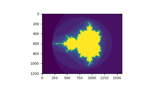
您可以查看以下示例,了解如何使用布尔索引生成 Mandelbrot 集 的图像。
>>> import numpy as np
>>> import matplotlib.pyplot as plt
>>> def mandelbrot(h, w, maxit=20, r=2):
...     """Returns an image of the Mandelbrot fractal of size (h,w)."""
...     x = np.linspace(-2.5, 1.5, 4*h+1)
...     y = np.linspace(-1.5, 1.5, 3*w+1)
...     A, B = np.meshgrid(x, y)
...     C = A + B*1j
...     z = np.zeros_like(C)
...     divtime = maxit + np.zeros(z.shape, dtype=int)
...
...     for i in range(maxit):
...         z = z**2 + C
...         diverge = abs(z) > r                    # who is diverging
...         div_now = diverge & (divtime == maxit)  # who is diverging now
...         divtime[div_now] = i                    # note when
...         z[diverge] = r                          # avoid diverging too much
...
...     return divtime
>>> plt.clf()
>>> plt.imshow(mandelbrot(400, 400))
第二种使用布尔值进行索引的方式更类似于整数索引;对于数组的每个维度,我们提供一个 1D 布尔数组来选择我们想要的切片。
>>> a = np.arange(12).reshape(3, 4)
>>> b1 = np.array([False, True, True])         # first dim selection
>>> b2 = np.array([True, False, True, False])  # second dim selection
>>>
>>> a[b1, :]                                   # selecting rows
array([[ 4,  5,  6,  7],
       [ 8,  9, 10, 11]])
>>>
>>> a[b1]                                      # same thing
array([[ 4,  5,  6,  7],
       [ 8,  9, 10, 11]])
>>>
>>> a[:, b2]                                   # selecting columns
array([[ 0,  2],
       [ 4,  6],
       [ 8, 10]])
>>>
>>> a[b1, b2]                                  # a weird thing to do
array([ 4, 10])
请注意,一维布尔数组的长度必须与您想要切片的维度(或轴)的长度一致。在前面的示例中,b1 的长度为 3(a 中的行数),而 b2(长度为 4)适合索引 a 的第二个轴(列)。
ix_() 函数#
ix_ 函数可用于组合不同的向量,以便获得每个 n 元组的结果。例如,如果您想计算从每个向量 a、b 和 c 中取出的所有三元组的 a+b*c
>>> a = np.array([2, 3, 4, 5])
>>> b = np.array([8, 5, 4])
>>> c = np.array([5, 4, 6, 8, 3])
>>> ax, bx, cx = np.ix_(a, b, c)
>>> ax
array([[[2]],

       [[3]],

       [[4]],

       [[5]]])
>>> bx
array([[[8],
        [5],
        [4]]])
>>> cx
array([[[5, 4, 6, 8, 3]]])
>>> ax.shape, bx.shape, cx.shape
((4, 1, 1), (1, 3, 1), (1, 1, 5))
>>> result = ax + bx * cx
>>> result
array([[[42, 34, 50, 66, 26],
        [27, 22, 32, 42, 17],
        [22, 18, 26, 34, 14]],

       [[43, 35, 51, 67, 27],
        [28, 23, 33, 43, 18],
        [23, 19, 27, 35, 15]],

       [[44, 36, 52, 68, 28],
        [29, 24, 34, 44, 19],
        [24, 20, 28, 36, 16]],

       [[45, 37, 53, 69, 29],
        [30, 25, 35, 45, 20],
        [25, 21, 29, 37, 17]]])
>>> result[3, 2, 4]
17
>>> a[3] + b[2] * c[4]
17
您也可以按如下方式实现 reduce
>>> def ufunc_reduce(ufct, *vectors):
...    vs = np.ix_(*vectors)
...    r = ufct.identity
...    for v in vs:
...        r = ufct(r, v)
...    return r
然后像这样使用它
>>> ufunc_reduce(np.add, a, b, c)
array([[[15, 14, 16, 18, 13],
        [12, 11, 13, 15, 10],
        [11, 10, 12, 14,  9]],

       [[16, 15, 17, 19, 14],
        [13, 12, 14, 16, 11],
        [12, 11, 13, 15, 10]],

       [[17, 16, 18, 20, 15],
        [14, 13, 15, 17, 12],
        [13, 12, 14, 16, 11]],

       [[18, 17, 19, 21, 16],
        [15, 14, 16, 18, 13],
        [14, 13, 15, 17, 12]]])
与普通的 ufunc.reduce 相比,这种 reduce 版本的优势在于它利用了 广播规则,从而避免创建大小等于输出大小乘以向量数量的参数数组。
字符串索引#
参阅 结构化数组。
技巧和窍门#
这里我们列出了一些简短而有用的技巧。
“自动”重塑#
要改变数组的维度,您可以省略其中一个大小,它将自动推导出来
>>> a = np.arange(30)
>>> b = a.reshape((2, -1, 3))  # -1 means "whatever is needed"
>>> b.shape
(2, 5, 3)
>>> b
array([[[ 0,  1,  2],
        [ 3,  4,  5],
        [ 6,  7,  8],
        [ 9, 10, 11],
        [12, 13, 14]],

       [[15, 16, 17],
        [18, 19, 20],
        [21, 22, 23],
        [24, 25, 26],
        [27, 28, 29]]])
向量堆叠#
我们如何从一个等长行向量列表构造一个二维数组?在 MATLAB 中这很容易:如果 x 和 y 是两个相同长度的向量,你只需要做 m=[x;y]。在 NumPy 中,这通过函数 column_stack, dstack, hstack 和 vstack 来实现,取决于堆叠的维度。例如
>>> x = np.arange(0, 10, 2)
>>> y = np.arange(5)
>>> m = np.vstack([x, y])
>>> m
array([[0, 2, 4, 6, 8],
       [0, 1, 2, 3, 4]])
>>> xy = np.hstack([x, y])
>>> xy
array([0, 2, 4, 6, 8, 0, 1, 2, 3, 4])
这些函数在超过二维时的逻辑可能比较奇怪。
另请参阅
直方图#
NumPy 的 histogram 函数应用于一个数组,返回一对向量:数组的直方图和 bin 边缘的向量。请注意:matplotlib 也有一个构建直方图的函数(称为 hist,如 Matlab 中一样),它与 NumPy 中的不同。主要区别在于 pylab.hist 会自动绘制直方图,而 numpy.histogram 只生成数据。
>>> import numpy as np
>>> rg = np.random.default_rng(1)
>>> import matplotlib.pyplot as plt
>>> # Build a vector of 10000 normal deviates with variance 0.5^2 and mean 2
>>> mu, sigma = 2, 0.5
>>> v = rg.normal(mu, sigma, 10000)
>>> # Plot a normalized histogram with 50 bins
>>> plt.hist(v, bins=50, density=True)       # matplotlib version (plot)
(array...)
>>> # Compute the histogram with numpy and then plot it
>>> (n, bins) = np.histogram(v, bins=50, density=True)  # NumPy version (no plot)
>>> plt.plot(.5 * (bins[1:] + bins[:-1]), n)
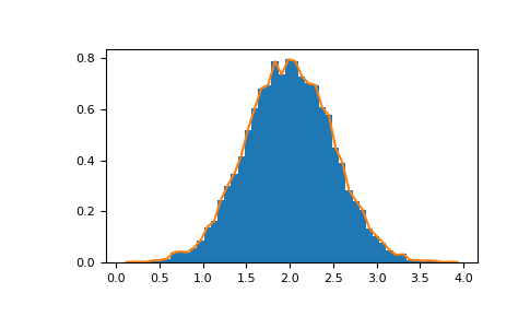
对于 Matplotlib >=3.4,您还可以使用 plt.stairs(n, bins)。