numpy.histogram#
- numpy.histogram(a, bins=10, range=None, density=None, weights=None)[源代码]#
计算数据集的直方图。
- 参数:
- a类数组对象
输入数据。直方图是在展平的数组上计算的。
- binsint 或标量序列或字符串,可选
如果 bins 是一个整数,它定义了给定范围内的等宽分箱数(默认为 10)。如果 bins 是一个序列,它定义了一个单调递增的分箱边界数组,包括最右侧的边界,允许非均匀分箱宽度。
如果 bins 是一个字符串,它定义了用于计算最佳分箱宽度的算法,如
histogram_bin_edges所定义。- range(float, float),可选
分箱的下限和上限。如果未提供,则 range 简单地为
(a.min(), a.max())。范围之外的值将被忽略。范围的第一个元素必须小于或等于第二个元素。range 也会影响自动分箱的计算。虽然分箱宽度是根据 range 内的实际数据计算为最优的,但分箱数量将填充整个范围,包括不包含数据的部分。- weightsarray_like, optional
一个权重数组,形状与 a 相同。 a 中的每个值仅将其相关的权重计入分箱计数(而不是 1)。如果 density 为 True,则权重会被归一化,使得密度在范围内的积分保持为 1。请注意,weights 的
dtype将成为返回的累加器(hist)的dtype,因此它必须足够大以容纳累积值。- densitybool,可选
如果为
False,则结果将包含每个分箱中的样本数。如果为True,则结果是概率 *密度* 函数在分箱处的值,归一化使得在范围内的 *积分* 为 1。请注意,直方图值之和不等于 1,除非选择了宽度为 1 的分箱;它不是概率 *质量* 函数。
- 返回:
- histarray
直方图的值。有关可能的语义的描述,请参见 density 和 weights。如果给定了 weights,则
hist.dtype将从 weights 中获取。- bin_edgesdtype 为 float 的 array
返回分箱边界
(length(hist)+1)。
备注
除最后一个(最右侧)分箱外,所有分箱都是半开区间。换句话说,如果 bins 是
[1, 2, 3, 4]
那么第一个分箱是
[1, 2)(包含 1,但不包含 2),第二个分箱是[2, 3)。然而,最后一个分箱是[3, 4],它 *包含* 4。示例
>>> import numpy as np
>>> np.histogram([1, 2, 1], bins=[0, 1, 2, 3])
(array([0, 2, 1]), array([0, 1, 2, 3]))
>>> np.histogram(np.arange(4), bins=np.arange(5), density=True)
(array([0.25, 0.25, 0.25, 0.25]), array([0, 1, 2, 3, 4]))
>>> np.histogram([[1, 2, 1], [1, 0, 1]], bins=[0,1,2,3])
(array([1, 4, 1]), array([0, 1, 2, 3]))
>>> a = np.arange(5)
>>> hist, bin_edges = np.histogram(a, density=True)
>>> hist
array([0.5, 0. , 0.5, 0. , 0. , 0.5, 0. , 0.5, 0. , 0.5])
>>> hist.sum()
2.4999999999999996
>>> np.sum(hist * np.diff(bin_edges))
1.0
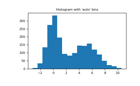
使用具有 2000 个点的 2 个峰随机数据的自动分箱选择方法示例。
import matplotlib.pyplot as plt
import numpy as np

rng = np.random.RandomState(10)  # deterministic random data
a = np.hstack((rng.normal(size=1000),
               rng.normal(loc=5, scale=2, size=1000)))
plt.hist(a, bins='auto')  # arguments are passed to np.histogram
plt.title("Histogram with 'auto' bins")
plt.show()