numpy.hanning#

numpy.hanning(M)[源代码]#

返回 Hanning 窗。

Hanning 窗是通过加权余弦形成的锥形函数。

参数:

Mint: 输出窗口中的点数。如果为零或负数，则返回空数组。

返回:

outndarray, shape(M,): 该窗，其最大值被归一化为一（当 M 是奇数时，值为一）。

另请参阅

bartlett, blackman, hamming, kaiser

备注

Hanning 窗定义为：

\[w(n) = 0.5 - 0.5\cos\left(\frac{2\pi{n}}{M-1}\right) \qquad 0 \leq n \leq M-1\]

Hanning 窗以奥地利气象学家 Julius von Hann 的名字命名。它也被称为余弦钟形（Cosine Bell）。有些作者更喜欢称其为 Hann 窗，以避免与非常相似的 Hamming 窗混淆。

关于 Hanning 窗的大多数引用都来自信号处理文献，其中它被用作许多平滑值的窗函数之一。它也被称为“去旁瓣”（apodization，意思是“去除脚”，即平滑采样信号开头和结尾处的间断）或锥形函数。

参考

[1]

Blackman, R.B. and Tukey, J.W., (1958) The measurement of power spectra, Dover Publications, New York.

[2]

E.R. Kanasewich, “Time Sequence Analysis in Geophysics”, The University of Alberta Press, 1975, pp. 106-108。

[3]

维基百科，“窗口函数”，https://en.wikipedia.org/wiki/Window_function

[4]

W.H. Press, B.P. Flannery, S.A. Teukolsky, and W.T. Vetterling, “Numerical Recipes”, Cambridge University Press, 1986, page 425。

示例

>>> import numpy as np
>>> np.hanning(12)
array([0.        , 0.07937323, 0.29229249, 0.57115742, 0.82743037,
       0.97974649, 0.97974649, 0.82743037, 0.57115742, 0.29229249,
       0.07937323, 0.        ])

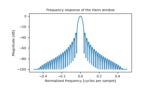
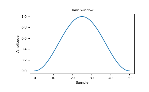
绘制窗口及其频率响应。

import matplotlib.pyplot as plt
from numpy.fft import fft, fftshift
window = np.hanning(51)
plt.plot(window)
plt.title("Hann window")
plt.ylabel("Amplitude")
plt.xlabel("Sample")
plt.show()

plt.figure()
A = fft(window, 2048) / 25.5
mag = np.abs(fftshift(A))
freq = np.linspace(-0.5, 0.5, len(A))
with np.errstate(divide='ignore', invalid='ignore'):
    response = 20 * np.log10(mag)
response = np.clip(response, -100, 100)
plt.plot(freq, response)
plt.title("Frequency response of the Hann window")
plt.ylabel("Magnitude [dB]")
plt.xlabel("Normalized frequency [cycles per sample]")
plt.axis('tight')
plt.show()