
X射线图像处理#
本教程演示如何使用NumPy、imageio、Matplotlib和SciPy读取和处理X射线图像。您将学习如何加载医学图像,聚焦于特定部分,并使用高斯、拉普拉斯-高斯、Sobel和Canny滤波器进行边缘检测,从而直观地比较它们。
X射线图像分析可以成为您数据分析和机器学习工作流程的一部分,例如,当您构建一个算法来帮助检测肺炎时,作为Kaggle竞赛的一部分。在医疗保健行业,医学图像处理和分析尤其重要,因为据估计图像至少占所有医疗数据的90%。
您将使用由美国国立卫生研究院 (NIH)提供的ChestX-ray8数据集中的放射图像。ChestX-ray8包含来自30,000多名患者的超过100,000张PNG格式的去身份化X射线图像。您可以在NIH的公共Box仓库的/images文件夹中找到ChestX-ray8的文件。(更多详情,请参阅2017年在CVPR(计算机视觉会议)上发表的研究论文。)
为方便起见,少量PNG图像已保存到本教程的仓库中,位于tutorial-x-ray-image-processing/下,因为ChestX-ray8包含数千兆字节的数据,您可能会发现分批下载它具有挑战性。

先决条件#
读者应具备一些Python、NumPy数组和Matplotlib的知识。为了复习,您可以学习Python和Matplotlib PyPlot教程,以及NumPy快速入门。
本教程使用以下包
imageio用于读写图像数据。医疗保健行业通常使用DICOM格式进行医学成像,而imageio应该非常适合读取该格式。为简单起见,本教程中您将使用PNG文件。
Matplotlib用于数据可视化。
本教程可以在隔离环境中本地运行,例如Virtualenv或conda。您可以使用Jupyter Notebook或JupyterLab来运行每个笔记本单元格。
目录#
使用
imageio检查X射线图像将图像合并成多维数组以展示进展
使用拉普拉斯-高斯、高斯梯度、Sobel和Canny滤波器进行边缘检测
使用
np.where()将掩码应用于X射线图像比较结果
使用imageio检查X射线图像#
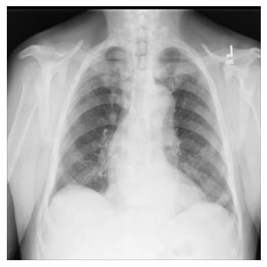
让我们从一个简单的例子开始,只使用ChestX-ray8数据集中的一张X射线图像。
文件—00000011_001.png—已为您下载并保存在/tutorial-x-ray-image-processing文件夹中。
1. 使用imageio加载图像
import os
import imageio

DIR = "tutorial-x-ray-image-processing"

xray_image = imageio.v3.imread(os.path.join(DIR, "00000011_001.png"))
2. 检查其形状是否为1024x1024像素,并且数组由8位整数组成
print(xray_image.shape)
print(xray_image.dtype)
(1024, 1024)
uint8
3. 导入matplotlib并以灰度色彩映射显示图像
import matplotlib.pyplot as plt

plt.imshow(xray_image, cmap="gray")
plt.axis("off")
plt.show()
将图像合并成多维数组以展示进展#
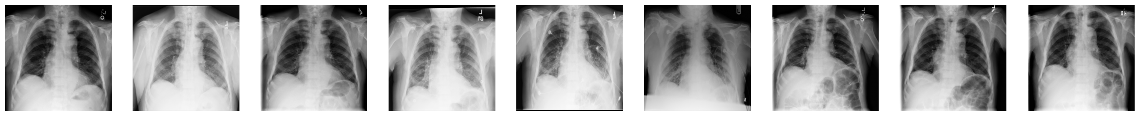
在下一个示例中,您将使用从ChestX-ray8数据集下载并提取的9张1024x1024像素的X射线图像,而不是1张图像。它们的编号从...000.png到...008.png,我们假设它们属于同一位患者。
1. 导入NumPy,读取每张X射线图像,并创建一个三维数组,其中第一个维度对应于图像编号
import numpy as np
num_imgs = 9

combined_xray_images_1 = np.array(
    [imageio.v3.imread(os.path.join(DIR, f"00000011_00{i}.png")) for i in range(num_imgs)]
)
2. 检查包含9张堆叠图像的新X射线图像数组的形状
combined_xray_images_1.shape
(9, 1024, 1024)
请注意,第一个维度中的形状与num_imgs匹配,因此combined_xray_images_1数组可以解释为2D图像的堆栈。
3. 您现在可以使用Matplotlib将每帧并排绘制,以显示“健康进展”
fig, axes = plt.subplots(nrows=1, ncols=num_imgs, figsize=(30, 30))

for img, ax in zip(combined_xray_images_1, axes):
    ax.imshow(img, cmap='gray')
    ax.axis('off')
4. 此外,将进展显示为动画也很有帮助。让我们使用imageio.mimwrite()创建一个GIF文件并在笔记本中显示结果
GIF_PATH = os.path.join(DIR, "xray_image.gif")
imageio.mimwrite(GIF_PATH, combined_xray_images_1, format= ".gif", duration=1000)
这给了我们: 
使用拉普拉斯-高斯、高斯梯度、Sobel和Canny滤波器进行边缘检测#
在处理生物医学数据时,强调2D“边缘”以聚焦图像中的特定特征可能很有用。为此,使用图像梯度在检测颜色像素强度变化时特别有帮助。
带有高斯二阶导数的拉普拉斯滤波器#
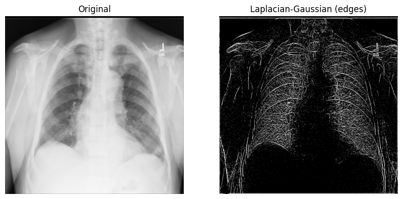
让我们从一个n维拉普拉斯滤波器(“拉普拉斯-高斯”)开始,该滤波器使用高斯二阶导数。这种拉普拉斯方法侧重于值强度快速变化的像素,并与高斯平滑相结合以去除噪声。让我们研究一下它在分析2D X射线图像中的作用。
拉普拉斯-高斯滤波器的实现相对简单:1)从SciPy导入
ndimage模块;2)调用scipy.ndimage.gaussian_laplace(),并带有一个sigma(标量)参数,该参数影响高斯滤波器的标准差(在下面的示例中您将使用1)
from scipy import ndimage

xray_image_laplace_gaussian = ndimage.gaussian_laplace(xray_image, sigma=1)
显示原始X射线图像和经过拉普拉斯-高斯滤波器处理的图像
fig, axes = plt.subplots(nrows=1, ncols=2, figsize=(10, 10))

axes[0].set_title("Original")
axes[0].imshow(xray_image, cmap="gray")
axes[1].set_title("Laplacian-Gaussian (edges)")
axes[1].imshow(xray_image_laplace_gaussian, cmap="gray")
for i in axes:
    i.axis("off")
plt.show()
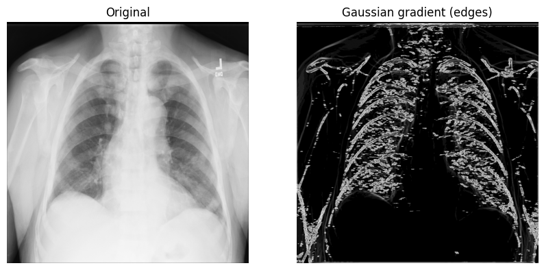
高斯梯度幅值方法#
另一种有用的边缘检测方法是高斯(梯度)滤波器。它使用高斯导数计算多维梯度幅值,并有助于去除高频图像分量。
1. 调用scipy.ndimage.gaussian_gradient_magnitude(),并带有一个sigma(标量)参数(用于标准差;在下面的示例中您将使用2)
x_ray_image_gaussian_gradient = ndimage.gaussian_gradient_magnitude(xray_image, sigma=2)
2. 显示原始X射线图像和经过高斯梯度滤波器处理的图像
fig, axes = plt.subplots(nrows=1, ncols=2, figsize=(10, 10))

axes[0].set_title("Original")
axes[0].imshow(xray_image, cmap="gray")
axes[1].set_title("Gaussian gradient (edges)")
axes[1].imshow(x_ray_image_gaussian_gradient, cmap="gray")
for i in axes:
    i.axis("off")
plt.show()
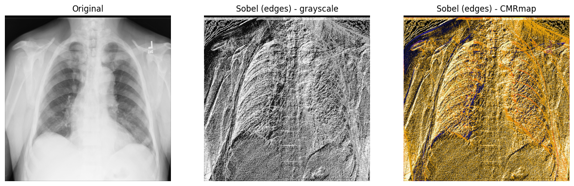
Sobel-Feldman算子(Sobel滤波器)#
为了找到2D X射线图像沿水平和垂直轴的高空间频率区域(边缘或边缘图),您可以使用Sobel-Feldman算子(Sobel滤波器)技术。Sobel滤波器通过卷积将两个3x3核矩阵(每个轴一个)应用于X射线。然后,使用勾股定理组合这两个点(梯度)以产生梯度幅值。
1. 在X射线的x轴和y轴上使用Sobel滤波器(scipy.ndimage.sobel())。然后,使用勾股定理和NumPy的np.hypot()计算x和y(应用Sobel滤波器后)之间的距离以获得幅值。最后,对重新缩放的图像进行归一化,使像素值介于0和255之间。
图像归一化遵循output_channel = 255.0 * (input_channel - min_value) / (max_value - min_value)公式。因为您使用的是灰度图像,所以只需归一化一个通道。
x_sobel = ndimage.sobel(xray_image, axis=0)
y_sobel = ndimage.sobel(xray_image, axis=1)

xray_image_sobel = np.hypot(x_sobel, y_sobel)

xray_image_sobel *= 255.0 / np.max(xray_image_sobel)
2. 将新图像数组的数据类型从float16更改为32位浮点格式,以使其与Matplotlib兼容
print("The data type - before: ", xray_image_sobel.dtype)

xray_image_sobel = xray_image_sobel.astype("float32")

print("The data type - after: ", xray_image_sobel.dtype)
The data type - before:  float16
The data type - after:  float32
3. 显示原始X射线图像和应用了Sobel“边缘”滤波器的图像。请注意,灰度图和CMRmap色彩映射都被用于帮助强调边缘。
fig, axes = plt.subplots(nrows=1, ncols=3, figsize=(15, 15))

axes[0].set_title("Original")
axes[0].imshow(xray_image, cmap="gray")
axes[1].set_title("Sobel (edges) - grayscale")
axes[1].imshow(xray_image_sobel, cmap="gray")
axes[2].set_title("Sobel (edges) - CMRmap")
axes[2].imshow(xray_image_sobel, cmap="CMRmap")
for i in axes:
    i.axis("off")
plt.show()
Canny滤波器#
您还可以考虑使用另一种著名的边缘检测滤波器,称为Canny滤波器。
首先,您应用一个高斯滤波器来去除图像中的噪声。在本例中,您使用的是傅里叶滤波器,它通过卷积过程平滑X射线。接下来,您对图像的2个轴分别应用Prewitt滤波器以帮助检测一些边缘——这将产生2个梯度值。与Sobel滤波器类似,Prewitt算子也通过卷积将两个3x3核矩阵(每个轴一个)应用于X射线。最后,您像之前一样,使用勾股定理计算两个梯度之间的幅值,并归一化图像。
1. 使用SciPy的傅里叶滤波器— scipy.ndimage.fourier_gaussian() —使用较小的sigma值去除X射线中的一些噪声。然后,使用scipy.ndimage.prewitt()计算两个梯度。接下来,使用NumPy的np.hypot()测量梯度之间的距离。最后,像之前一样,归一化重新缩放的图像。
fourier_gaussian = ndimage.fourier_gaussian(xray_image, sigma=0.05)

x_prewitt = ndimage.prewitt(fourier_gaussian, axis=0)
y_prewitt = ndimage.prewitt(fourier_gaussian, axis=1)

xray_image_canny = np.hypot(x_prewitt, y_prewitt)

xray_image_canny *= 255.0 / np.max(xray_image_canny)

print("The data type - ", xray_image_canny.dtype)
The data type - float64
2. 绘制原始X射线图像以及使用Canny滤波器技术检测到边缘的图像。可以使用prism、nipy_spectral和terrain Matplotlib色彩映射来强调边缘。
fig, axes = plt.subplots(nrows=1, ncols=4, figsize=(20, 15))

axes[0].set_title("Original")
axes[0].imshow(xray_image, cmap="gray")
axes[1].set_title("Canny (edges) - prism")
axes[1].imshow(xray_image_canny, cmap="prism")
axes[2].set_title("Canny (edges) - nipy_spectral")
axes[2].imshow(xray_image_canny, cmap="nipy_spectral")
axes[3].set_title("Canny (edges) - terrain")
axes[3].imshow(xray_image_canny, cmap="terrain")
for i in axes:
    i.axis("off")
plt.show()

使用np.where()将掩码应用于X射线图像#
为了筛选出X射线图像中的特定像素以帮助检测特定特征,您可以使用NumPy的np.where(condition: array_like (bool), x: array_like, y: ndarray)来应用掩码,当True时返回x,当False时返回y。
识别感兴趣区域——图像中的某些像素集——可能很有用,掩码作为与原始图像形状相同的布尔数组。
1. 检索您一直在处理的原始X射线图像中像素值的一些基本统计信息
print("The data type of the X-ray image is: ", xray_image.dtype)
print("The minimum pixel value is: ", np.min(xray_image))
print("The maximum pixel value is: ", np.max(xray_image))
print("The average pixel value is: ", np.mean(xray_image))
print("The median pixel value is: ", np.median(xray_image))
The data type of the X-ray image is:  uint8
The minimum pixel value is:  0
The maximum pixel value is:  255
The average pixel value is:  172.52233219146729
The median pixel value is:  195.0
2. 数组数据类型为uint8,最小/最大值结果表明X射线中使用了所有256种颜色(从0到255)。让我们使用ndimage.histogram()和Matplotlib可视化原始X射线图像的像素强度分布
pixel_intensity_distribution = ndimage.histogram(
    xray_image, min=np.min(xray_image), max=np.max(xray_image), bins=256
)

plt.plot(pixel_intensity_distribution)
plt.title("Pixel intensity distribution")
plt.show()
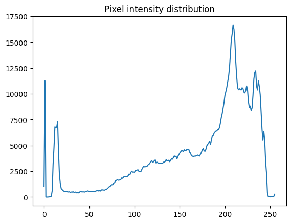
正如像素强度分布所示,存在许多低(约0到20之间)和非常高(约200到240之间)的像素值。
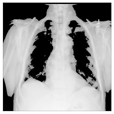
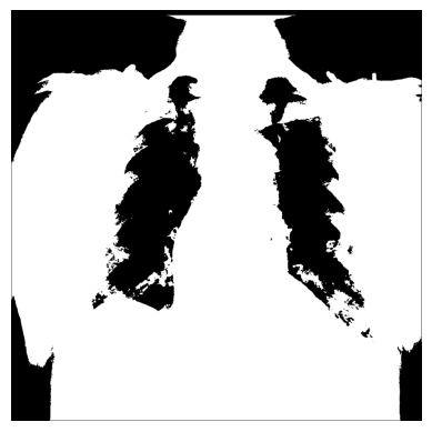
3. 您可以使用NumPy的np.where()创建不同的条件掩码——例如,我们只保留图像中像素值超过特定阈值的部分。
# The threshold is "greater than 150"
# Return the original image if true, `0` otherwise
xray_image_mask_noisy = np.where(xray_image > 150, xray_image, 0)

plt.imshow(xray_image_mask_noisy, cmap="gray")
plt.axis("off")
plt.show()
# The threshold is "greater than 150"
# Return `1` if true, `0` otherwise
xray_image_mask_less_noisy = np.where(xray_image > 150, 1, 0)

plt.imshow(xray_image_mask_less_noisy, cmap="gray")
plt.axis("off")
plt.show()
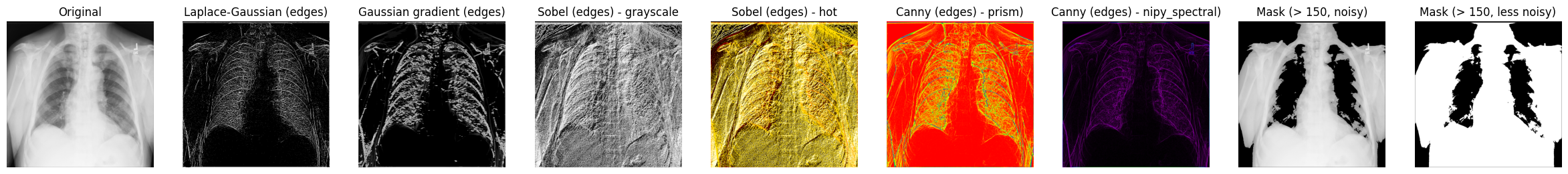
比较结果#
让我们展示一些您目前处理过的X射线图像结果
fig, axes = plt.subplots(nrows=1, ncols=9, figsize=(30, 30))

axes[0].set_title("Original")
axes[0].imshow(xray_image, cmap="gray")
axes[1].set_title("Laplace-Gaussian (edges)")
axes[1].imshow(xray_image_laplace_gaussian, cmap="gray")
axes[2].set_title("Gaussian gradient (edges)")
axes[2].imshow(x_ray_image_gaussian_gradient, cmap="gray")
axes[3].set_title("Sobel (edges) - grayscale")
axes[3].imshow(xray_image_sobel, cmap="gray")
axes[4].set_title("Sobel (edges) - hot")
axes[4].imshow(xray_image_sobel, cmap="hot")
axes[5].set_title("Canny (edges) - prism)")
axes[5].imshow(xray_image_canny, cmap="prism")
axes[6].set_title("Canny (edges) - nipy_spectral)")
axes[6].imshow(xray_image_canny, cmap="nipy_spectral")
axes[7].set_title("Mask (> 150, noisy)")
axes[7].imshow(xray_image_mask_noisy, cmap="gray")
axes[8].set_title("Mask (> 150, less noisy)")
axes[8].imshow(xray_image_mask_less_noisy, cmap="gray")
for i in axes:
    i.axis("off")
plt.show()
下一步#
如果您想使用自己的样本,可以使用此图像,或者在Openi数据库中搜索其他各种图像。Openi包含许多生物医学图像,如果您带宽较低和/或受限于可下载的数据量,它将特别有帮助。
要了解更多关于生物医学图像数据或简单边缘检测中的图像处理,您可能会发现以下材料有用
使用Scikit-Image和pydicom在Python中进行DICOM处理和分割(Radiology Data Quest)
使用Numpy和Scipy进行图像操作和处理(Scipy Lecture Notes)
强度值(演示文稿,DataCamp)
使用Raspberry Pi和Python进行对象检测(Maker Portal)
使用深度学习进行X射线数据准备和分割(Kaggle托管的Jupyter Notebook)
图像滤波(讲义,CS6670:计算机视觉,康奈尔大学)
使用Python和NumPy进行边缘检测(Towards Data Science)
使用Scikit-Image进行边缘检测(Data Carpentry)
图像梯度和梯度滤波(讲义,16-385 计算机视觉,卡内基梅隆大学)