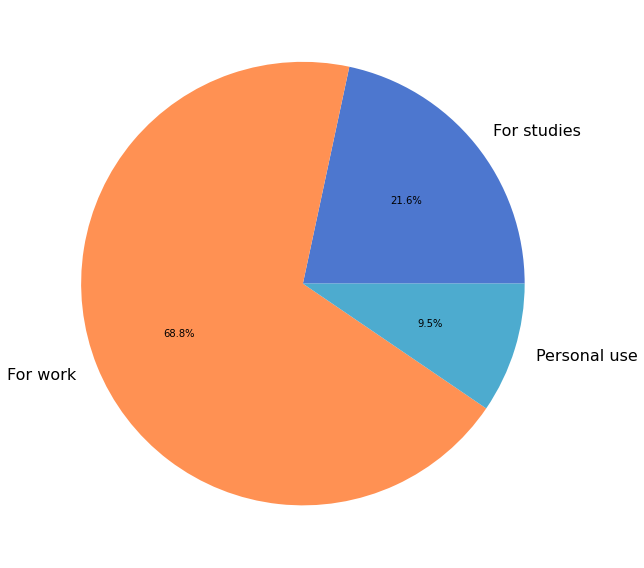
社区¶

NumPy 调查受访者人口统计信息的摘要。

fname = "data/2020/numpy_survey_results.tsv"
column_names = [
    'age', 'gender', 'lang', 'lang_other', 'country', 'degree', 'degree_other',
    'field_of_study', 'field_other', 'role', 'role_other', 'version', 
    'primary_use', 'programming_exp', 'numpy_exp', 'use_freq', 'components',
    'use_c_ext', 'prog_lang', 'prog_lang_other',
]
demographics_dtype = np.dtype({
    "names": column_names,
    "formats": ['<U600'] * len(column_names),
})

data = np.loadtxt(
    fname, delimiter='\t', skiprows=3, dtype=demographics_dtype, 
    usecols=range(11, 31), comments=None
)

glue('num_respondents', data.shape[0], display=False)

人口统计¶

年龄¶

在 1236 名调查受访者中，有 1089 名 (88%) 分享了他们的年龄。

age = data['age']
# Preprocessing
ignore_chars = ('', '> 40')
for value in ignore_chars:
    age = age[age != value]
age = age.astype(int)
# Distribution
bwidth = 10
bedges = np.arange(0, age.max() + bwidth, bwidth)
h, _ = np.histogram(age, bins=bedges)
h = 100 * h / h.sum()

fig, ax = plt.subplots(figsize=(12, 8))
x = np.arange(len(h))
ax.bar(x, h)
labels = [f"{low}-{high - 1}" for low, high in zip(bedges[:-1], bedges[1:])]
ax.set_xticks(x)
ax.set_xticklabels(labels)
fig.autofmt_xdate();
ax.set_title("Age Distribution of Survey Respondents");
ax.set_xlabel("Age (yrs)");
ax.set_ylabel("Percentage of Respondents");

glue('num_age_respondents', gluval(age.shape[0], data.shape[0]), display=False)

性别¶

在 1236 名调查受访者中，有 1100 名 (89%) 分享了他们的性别。

# Ignore empty fields and "prefer not to answer"
drop = np.logical_and(data['gender'] != '', data['gender'] != 'Prefer not to answer')
gender = data['gender'][drop]
labels, cnts = np.unique(gender, return_counts=True)

fig, ax = plt.subplots(figsize=(8, 8))
ax.pie(cnts, labels=labels, autopct='%1.1f%%')
ax.set_title("Gender Distribution of Survey Respondents");
fig.tight_layout()

glue('num_gender', gluval(gender.shape[0], data.shape[0]), display=False)

语言偏好¶

在 1236 名受访者中，有 1173 名 (95%) 分享了他们的首选语言。

# Ignore empty fields
lang = data['lang'][data['lang'] != '']
# Self-reported language
lang_other = data['lang_other'][data['lang_other'] != '']
lang_other = capitalize(lang_other)
lang = np.concatenate((lang, lang_other))
labels, cnts = np.unique(lang, return_counts=True)
cnts = 100 * cnts / cnts.sum()
I = np.argsort(cnts)[::-1]
labels, cnts = labels[I], cnts[I]

# Create a summary table
with open('_generated/language_preference_table.md', 'w') as of:
    of.write('| **Language** | **Preferred by % of Respondents** |\n')
    of.write('|--------------|-----------------------------------|\n')
    for lbl, percent in zip(labels, cnts):
        of.write(f'| {lbl} | {percent:1.1f} |\n')

glue('num_lang_pref', gluval(lang.shape[0], data.shape[0]), display=False)

点击显示/隐藏表格

语言	受访者偏好比例 (%)
英语	69.5
西班牙语	8.3
日语	6.7
其他	3.8
法语	2.8
葡萄牙语	2.0
俄语	1.9
德语	1.4
普通话	0.7
中文	0.5
阿拉伯语	0.3
孟加拉语	0.3
印地语	0.3
荷兰语	0.3
世界语	0.2
意大利语	0.2
泰米尔语	0.1
保加利亚语	0.1
加泰罗尼亚语	0.1
乌克兰语	0.1
捷克语	0.1
Python	0.1
挪威语	0.1
瑞典语	0.1
斯洛文尼亚语	0.1
印度尼西亚语	0.1
乌尔都语	0.1
罗马尼亚语	0.1
中文	0.1

居住国家¶

在 1236 名受访者中，有 1095 名 (89%) 分享了他们当前的居住国家。本次调查总共收到了来自 75 个国家的受访者。

以下图表显示了来自参与者数量最多的约 20 个国家的受访者相对数量。出于隐私原因，受访者数量少于一定数量的国家未包含在图中，而是列在随后的表格中。

# Preprocess data
country = data['country'][data['country'] != '']
country = strip(country)
# Distribution
labels, cnts = np.unique(country, return_counts=True)
# Privacy filter
num_resp = 10
cutoff = (cnts > num_resp)
plabels = np.concatenate((labels[cutoff], ['Other']))
pcnts = np.concatenate((cnts[cutoff], [cnts[~cutoff].sum()]))

fig, ax = plt.subplots(figsize=(8, 8))
ax.pie(pcnts, labels=plabels, autopct='%1.1f%%')
ax.set_title('Global Distribution of Respondents')
fig.tight_layout()

# Map countries to continents
import pycountry_convert as pc
cont_code_to_cont_name = {
    'NA': 'North America',
    'SA': 'South America',
    'AS': 'Asia',
    'EU': 'Europe',
    'AF': 'Africa',
    'OC': 'Oceania',
}
def country_to_continent(country_name):
    cc = pc.country_name_to_country_alpha2(country_name)
    cont_code = pc.country_alpha2_to_continent_code(cc)
    return cont_code_to_cont_name[cont_code]
c2c = np.vectorize(country_to_continent, otypes='U')

# Organize countries below the privacy cutoff by their continent
remaining_countries = labels[~cutoff]
continents = c2c(remaining_countries)
with open('_generated/countries_by_continent.md', 'w') as of:
    of.write('|  |  |\n')
    of.write('|---------------|-------------|\n')
    for continent in np.unique(continents):
        clist = remaining_countries[continents == continent]
        of.write(f"| **{continent}:** | {', '.join(clist)} |\n")

glue('num_unique_countries', len(labels), display=False)
glue(
    'num_country_respondents',
    gluval(country.shape[0], data.shape[0]),
    display=False
)


非洲	佛得角、埃及、加纳、肯尼亚、摩洛哥、尼日利亚、南非、多哥
亚洲	亚美尼亚、巴林、孟加拉国、香港、印度尼西亚、伊朗、以色列、马来西亚、尼泊尔、巴基斯坦、沙特阿拉伯、新加坡、斯里兰卡、台湾、泰国、土耳其
欧洲	阿尔巴尼亚、奥地利、白俄罗斯、波斯尼亚和黑塞哥维那、保加利亚、克罗地亚、捷克共和国、丹麦、爱沙尼亚、芬兰、希腊、匈牙利、爱尔兰、拉脱维亚、挪威、波兰、葡萄牙、罗马尼亚、斯洛伐克、斯洛文尼亚、瑞典、乌克兰
北美洲	哥斯达黎加、萨尔瓦多、墨西哥
大洋洲	新西兰
南美洲	玻利维亚、智利、厄瓜多尔、巴拉圭、秘鲁、乌拉圭、委内瑞拉

教育背景¶

有 1118 名 (90%) 受访者分享了他们的教育背景，涵盖了从高中毕业前到博士学位以及许多其他专业学位。下图总结了所报告的最常见学位类型的分布情况。

degree = data['degree'][data['degree'] != '']
labels, cnts = np.unique(degree, return_counts=True)

fig, ax = plt.subplots(figsize=(8, 8))
ax.pie(cnts, labels=labels, autopct='%1.1f%%', labeldistance=None)
ax.set_title("Distribution of Highest Degree Obtained by Respondents")
ax.legend()
fig.tight_layout()

glue('num_education', gluval(degree.shape[0], data.shape[0]), display=False)

职业角色¶

在 1106 名分享了自己职业的受访者中，有 464 名 (42%) 的身份是博士生、软件工程师或数据科学家。

role = data['role'][data['role'] != '']
labels, cnts = np.unique(role, return_counts=True)

# Sort results by number of selections
inds = np.argsort(cnts)
labels, cnts = labels[inds], cnts[inds]

fig, ax = plt.subplots(figsize=(12, 8))
ax.barh(np.arange(len(cnts)), cnts, align='center')
ax.set_yticks(np.arange(len(cnts)))
ax.set_yticklabels(labels)
ax.set_xlabel("Number of Respondents")
fig.tight_layout()

glue('num_occupation', role.shape[0], display=False)
glue(
    'num_top_3_categories',
    gluval(cnts[-3:].sum(), role.shape[0]),
    display=False,
)
glue('top_3_categories', f"{labels[-3]}, {labels[-2]}, or {labels[-1]}", display=False)

经验和使用情况¶

编程经验¶

有 63% 的受访者拥有丰富的编程经验，其中资深开发者（10 年以上）占主导地位。有趣的是，在使用 NumPy 方面，我们的受访者中自认为是初学者的人数明显多于经验丰富的用户。

fig, axes = plt.subplots(1, 2, figsize=(12, 6))
# Ascending order for figure
ind = np.array([-1, 0, 2, 3, 1])
for exp_data, ax in zip(('programming_exp', 'numpy_exp'), axes):
    # Analysis
    prog_exp = data[exp_data][data[exp_data] != '']
    labels, cnts = np.unique(prog_exp, return_counts=True)
    cnts = 100 * cnts / cnts.sum()
    labels, cnts = labels[ind], cnts[ind]
    # Generate text on general programming experience
    glue(f'{exp_data}_5plus_years', f"{cnts[-2:].sum():2.0f}%", display=False)
    # Plotting
    ax.bar(np.arange(len(cnts)), cnts)
    ax.set_xticks(np.arange(len(cnts)))
    ax.set_xticklabels(labels)
axes[0].set_title('General Programming Experience')
axes[0].set_ylabel('Percentage of Respondents')
axes[1].set_title('Experience with NumPy');
fig.autofmt_xdate();
fig.tight_layout();

编程语言¶

有 980 名 (79%) 调查参与者分享了他们使用其他编程语言的经验。有 67% 的受访者熟悉 C / C++，有 44% 的受访者熟悉 Matlab。

pl = data['prog_lang'][data['prog_lang'] != '']
num_respondents = len(pl)
glue('num_proglang_respondents', gluval(len(pl), data.shape[0]), display=False)

# Flatten & remove 'Other' write-in option
other = 'Other (please specify, using commas to separate individual entries)'
apl = []
for row in pl:
    if 'Other' in row:
        row = ','.join(row.split(',')[:-2])
        if len(row) < 1:
            continue
    apl.extend(row.split(','))
labels, cnts = np.unique(apl, return_counts=True)
cnts = 100 * cnts / num_respondents
I = np.argsort(cnts)
labels, cnts = labels[I], cnts[I]

fig, ax = plt.subplots(figsize=(12, 8))
ax.barh(np.arange(len(cnts)), cnts, align='center')
ax.set_yticks(np.arange(len(cnts)))
ax.set_yticklabels(labels)
ax.set_xlabel("Percentage of Respondents")
ax.set_title("Programming Language Familiarity")
fig.tight_layout()

# Highlight two most popular
glue('num_top_lang', f"{cnts[-1]:2.0f}%", display=False)
glue('top_lang', labels[-1], display=False)
glue('num_2nd_lang', f"{cnts[-2]:2.0f}%", display=False)
glue('second_lang', labels[-2], display=False)

有 186 名 (19%) 受访者表示熟悉上述列表之外的计算机语言。其中，Rust 最受欢迎，有 39 名 (4%) 受访者使用此语言。其他报告的语言列表可在下方找到（点击展开）。

['apl' 'asm' 'assembler' 'bash' 'basic' 'befunge' 'brainfuck' 'chapel'
 'cobol' 'common lisp' 'crystal' 'cuda' 'dart' 'delphi pascal' 'elisp'
 'emacs lisp' 'fame' 'flutter' 'go' 'golang' 'groovy' 'haskell' 'html'
 'idl' 'igor pro' 'it counts!' 'kotlin' 'kuin' 'labview' 'latex' 'lisp'
 'logo' 'lua' 'macaulay2' 'mathematica' 'modellica' 'netlogo' 'nim' 'node'
 'oberon' 'ocaml' 'octave' 'pascal' 'perl' 'perl 5' 'php' 'postscript'
 'processing' 'prolog' 'python' 'q#' 'racket' 'rust' 'sas' 'scala'
 'scheme' 'shell' 'shellscript' 'smalltalk' 'solidity' 'spp' 'sql' 'swift'
 'tcl' 'turbo pascal' 'turtle' 'typescript' 'unix'
 'various assembly languages' 'vba' 'visual basic'
 'visual basic for applications' 'visual basic 🥳' 'wolfram' 'xslt']

NumPy 版本¶

NumPy 1.18 是调查进行时最新的稳定版本。有 12.3% 的受访者表示他们主要使用较旧的 NumPy 版本。

vers = data['version'][data['version'] != '']
labels, cnts = np.unique(vers, return_counts=True)

fig, ax = plt.subplots(figsize=(12, 8))
ax.pie(cnts, labels=labels, autopct='%1.1f%%')
fig.tight_layout()

# Percentage of users that use older versions
older_version_usage = 100 * cnts[-4:-1].sum() / cnts.sum()
glue('older_version_usage', f"{older_version_usage:1.1f}", display=False)

主要用例¶

有 1072 名 (87%) 受访者提供了他们使用 NumPy 的主要场景信息。

uses = data['primary_use'][data['primary_use'] != '']
labels, cnts = np.unique(uses, return_counts=True)

fig, ax = plt.subplots(figsize=(12, 8))
ax.pie(cnts, labels=labels, autopct='%1.1f%%')
fig.tight_layout()

glue(
    'num_primary_use_respondents',
    gluval(uses.shape[0], data.shape[0]),
    display=False
)

使用频率¶

有 1073 名 (87%) 受访者提供了他们使用 NumPy 的频率信息。

use_freq = data['use_freq'][data['use_freq'] != '']
labels, cnts = np.unique(use_freq, return_counts=True)

fig, ax = plt.subplots(figsize=(12, 8))
ax.pie(cnts, labels=labels, autopct='%1.1f%%')
fig.tight_layout()

glue('num_freq_respondents', gluval(use_freq.shape[0], data.shape[0]), display=False)

NumPy 组件¶

NumPy 包含许多用于特定科学计算任务的包，例如随机数生成或傅里叶分析。下图显示了报告使用每个 NumPy 子包的受访者百分比。

components = data['components'][data['components'] != '']
num_respondents = len(components)
# Process components field
all_components = []
for row in components:
    all_components.extend(row.split(','))
all_components = np.array(all_components)
labels, cnts = np.unique(all_components, return_counts=True)
# Descending order
I = np.argsort(cnts)
labels, cnts = labels[I], cnts[I]
cnts = 100 * cnts / num_respondents

fig, ax = plt.subplots(figsize=(12, 8))
ax.barh(np.arange(len(cnts)), cnts, align='center')
ax.set_yticks(np.arange(len(cnts)))
ax.set_yticklabels(labels)
ax.set_xlabel("Percentage of Respondents")
ax.set_title("Use-Frequency of NumPy Sub-Packages")
fig.tight_layout()

NumPy C 扩展¶

有 863 名参与者分享了他们（或其组织）是否通过 NumPy C-API 使用自定义 C 扩展（不包括 Cython）。

uses_c_ext = data['use_c_ext']
labels, cnts = np.unique(uses_c_ext, return_counts=True)
labels[0] = 'No response'

fig, ax = plt.subplots(figsize=(8, 8))
ax.pie(cnts, labels=labels, autopct='%1.1f%%')
fig.tight_layout()

glue('num_c_ext', np.sum(uses_c_ext != ''), display=False)

2020 年调查结果

贡献