本教程演示了如何从头开始使用 NumPy 构建一个简单的 前馈神经网络(带有一个隐藏层)并对其进行训练,以识别手写数字图像。
您的深度学习模型——作为最基本的人工神经网络之一,类似于最初的 多层感知机——将从 MNIST 数据集中学习对 0 到 9 的数字进行分类。该数据集包含 60,000 张训练图像和 10,000 张测试图像以及相应的标签。每张训练和测试图像的大小为 784(或 28x28 像素)——这将是您神经网络的输入。
基于图像输入及其标签(监督学习),您的神经网络将通过前向传播和反向传播(反向模式微分)进行训练,以学习它们的特征。网络的最终输出是一个包含 10 个分数的向量——每个分数对应一个手写数字图像。您还将评估模型在测试集上分类图像的准确性。
本教程改编自 Andrew Trask 的作品(经作者许可)。
先决条件
读者应具备 Python、NumPy 数组操作和线性代数方面的知识。此外,您还应该熟悉 深度学习 的主要概念。
为了复习,您可以参考 Python 和 n 维数组上的线性代数 教程。
建议您阅读 Yann LeCun、Yoshua Bengio 和 Geoffrey Hinton(被誉为该领域的先驱)于 2015 年发表的 深度学习 论文。您还应该考虑阅读 Andrew Trask 的 Grokking Deep Learning,该书使用 NumPy 教授深度学习。
除了 NumPy 之外,您还将使用以下 Python 标准模块进行数据加载和处理:
urllib用于 URL 处理request用于 URL 打开gzip用于 gzip 文件解压pickle用于处理 pickle 文件格式以及
Matplotlib 用于数据可视化
本教程可以在隔离环境中本地运行,例如 Virtualenv 或 conda。您可以使用 Jupyter Notebook 或 JupyterLab 来运行每个 notebook 单元格。别忘了 设置 NumPy 和 Matplotlib。
目录
加载 MNIST 数据集
预处理数据集
从头开始构建和训练小型神经网络
下一步
1. 加载 MNIST 数据集
在本节中,您将下载由 Yann LeCun 研究团队最初开发的 MNIST 数据集压缩文件。(MNIST 数据集的更多详细信息可在 Kaggle 上找到。)然后,您将使用内置的 Python 模块将它们转换为 4 个 NumPy 数组类型的文件。最后,您将把数组分割成训练集和测试集。
1. 定义一个变量,将 MNIST 数据集的训练/测试图像/标签名称存储在一个列表中
data_sources = {
    "training_images": "train-images-idx3-ubyte.gz",  # 60,000 training images.
    "test_images": "t10k-images-idx3-ubyte.gz",  # 10,000 test images.
    "training_labels": "train-labels-idx1-ubyte.gz",  # 60,000 training labels.
    "test_labels": "t10k-labels-idx1-ubyte.gz",  # 10,000 test labels.
}
2. 加载数据。首先检查数据是否已存储在本地;如果未存储,则下载。
import requests
import os

data_dir = "../_data"
os.makedirs(data_dir, exist_ok=True)

base_url = "https://ossci-datasets.s3.amazonaws.com/mnist/"

for fname in data_sources.values():
    fpath = os.path.join(data_dir, fname)
    if not os.path.exists(fpath):
        print("Downloading file: " + fname)
        resp = requests.get(base_url + fname, stream=True, **request_opts)
        resp.raise_for_status()  # Ensure download was succesful
        with open(fpath, "wb") as fh:
            for chunk in resp.iter_content(chunk_size=128):
                fh.write(chunk)
Downloading file: train-images-idx3-ubyte.gz
Downloading file: t10k-images-idx3-ubyte.gz
Downloading file: train-labels-idx1-ubyte.gz
Downloading file: t10k-labels-idx1-ubyte.gz
3. 解压 4 个文件,创建 4 个 ndarrays,并将它们保存在一个字典中。原始图像的大小为 28x28,神经网络通常期望一维向量输入;因此,您还需要通过将 28 乘以 28(784)来重塑图像。
import gzip
import numpy as np

mnist_dataset = {}

# Images
for key in ("training_images", "test_images"):
    with gzip.open(os.path.join(data_dir, data_sources[key]), "rb") as mnist_file:
        mnist_dataset[key] = np.frombuffer(
            mnist_file.read(), np.uint8, offset=16
        ).reshape(-1, 28 * 28)
# Labels
for key in ("training_labels", "test_labels"):
    with gzip.open(os.path.join(data_dir, data_sources[key]), "rb") as mnist_file:
        mnist_dataset[key] = np.frombuffer(mnist_file.read(), np.uint8, offset=8)
4. 使用标准的 `x` 表示数据,`y` 表示标签,将数据分割成训练集和测试集,分别将训练集和测试集的图像称为 `x_train` 和 `x_test`,将标签称为 `y_train` 和 `y_test`。
x_train, y_train, x_test, y_test = (
    mnist_dataset["training_images"],
    mnist_dataset["training_labels"],
    mnist_dataset["test_images"],
    mnist_dataset["test_labels"],
)
5. 您可以确认训练集和测试集的图像数组形状分别为 `(60000, 784)` 和 `(10000, 784)`,标签的形状分别为 `(60000,)` 和 `(10000,)`。
print(
    "The shape of training images: {} and training labels: {}".format(
        x_train.shape, y_train.shape
    )
)
print(
    "The shape of test images: {} and test labels: {}".format(
        x_test.shape, y_test.shape
    )
)
The shape of training images: (60000, 784) and training labels: (60000,)
The shape of test images: (10000, 784) and test labels: (10000,)
6. 您可以使用 Matplotlib 检查一些图像。
import matplotlib.pyplot as plt

# Take the 60,000th image (indexed at 59,999) from the training set,
# reshape from (784, ) to (28, 28) to have a valid shape for displaying purposes.
mnist_image = x_train[59999, :].reshape(28, 28)
# Set the color mapping to grayscale to have a black background.
plt.imshow(mnist_image, cmap="gray")
# Display the image.
plt.show()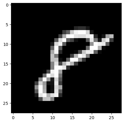
# Display 5 random images from the training set.
num_examples = 5
seed = 147197952744
rng = np.random.default_rng(seed)

fig, axes = plt.subplots(1, num_examples)
for sample, ax in zip(rng.choice(x_train, size=num_examples, replace=False), axes):
    ax.imshow(sample.reshape(28, 28), cmap="gray")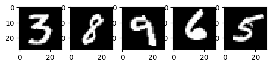
以上是 MNIST 训练集中的五张图像。展示了各种手绘的阿拉伯数字,具体值在每次运行代码时随机选择。
注意:您还可以通过打印 `x_train[59999]` 将样本图像可视化为数组。在这里,`59999` 是您的第 60,000 个训练图像样本(`0` 是您的第一个)。您的输出将很长,并且应该包含一个 8 位整数数组。
...
         0,   0,  38,  48,  48,  22,   0,   0,   0,   0,   0,   0,   0,
         0,   0,   0,   0,   0,   0,   0,   0,   0,   0,   0,   0,   0,
         0,  62,  97, 198, 243, 254, 254, 212,  27,   0,   0,   0,   0,
...
# Display the label of the 60,000th image (indexed at 59,999) from the training set.
y_train[59999]np.uint8(8)2. 预处理数据
神经网络可以处理浮点类型张量(多维数组)形式的输入。在预处理数据时,您应该考虑以下过程:向量化和转换为浮点格式。
由于 MNIST 数据已经向量化,并且数组的 `dtype` 为 `uint8`,因此您的下一个挑战是将其转换为浮点格式,例如 `float64`(双精度)。
实际上,您可以根据您的目标使用不同类型的浮点精度,有关更多信息,请参阅 Nvidia 和 Google Cloud 的博客文章。
将图像数据转换为浮点格式
图像数据包含 8 位整数,编码在 [0, 255] 区间内,颜色值在 0 到 255 之间。
您将通过除以 255 将它们标准化为 [0, 1] 区间的浮点数组。
1. 检查向量化图像数据的类型是否为 `uint8`。
print("The data type of training images: {}".format(x_train.dtype))
print("The data type of test images: {}".format(x_test.dtype))
The data type of training images: uint8
The data type of test images: uint8
2. 通过除以 255(从而将数据类型从 `uint8` 提升到 `float64`)来标准化数组,然后分别将训练和测试图像数据变量——`x_train` 和 `x_test`——赋值给 `training_images` 和 `train_labels`。为了在此示例中减少模型训练和评估时间,仅使用了训练和测试图像的子集。`training_images` 和 `test_images` 分别只包含 1,000 个样本,而完整的训练集和测试集分别为 60,000 和 10,000 张图像。这些值可以通过更改下面的 `training_sample` 和 `test_sample` 来控制,最高可达其最大值 60,000 和 10,000。
training_sample, test_sample = 1000, 1000
training_images = x_train[0:training_sample] / 255
test_images = x_test[0:test_sample] / 255
3. 确认图像数据已更改为浮点格式。
print("The data type of training images: {}".format(training_images.dtype))
print("The data type of test images: {}".format(test_images.dtype))
The data type of training images: float64
The data type of test images: float64
注意:您还可以通过在 notebook 单元格中打印 `training_images[0]` 来检查标准化是否成功。您的长输出应包含一个浮点数数组。
...
       0.        , 0.        , 0.01176471, 0.07058824, 0.07058824,
       0.07058824, 0.49411765, 0.53333333, 0.68627451, 0.10196078,
       0.65098039, 1.        , 0.96862745, 0.49803922, 0.        ,
...
将标签通过分类/独热编码转换为浮点数
您将使用独热编码,使用 `np.zeros()` 将每个数字标签嵌入一个全零向量,并在标签索引处放置 `1`。结果是,您的标签数据将是数组,其中每个图像标签的位置为 `1.0`(或 `1.`)。
由于总共有 10 个标签(从 0 到 9),您的数组将类似于:
array([0., 0., 0., 0., 0., 1., 0., 0., 0., 0.])1. 确认图像标签数据的类型是 `uint8` 整数。
print("The data type of training labels: {}".format(y_train.dtype))
print("The data type of test labels: {}".format(y_test.dtype))
The data type of training labels: uint8
The data type of test labels: uint8
2. 定义一个执行数组独热编码的函数。
def one_hot_encoding(labels, dimension=10):
    # Define a one-hot variable for an all-zero vector
    # with 10 dimensions (number labels from 0 to 9).
    one_hot_labels = labels[..., None] == np.arange(dimension)[None]
    # Return one-hot encoded labels.
    return one_hot_labels.astype(np.float64)
3. 编码标签并将值赋给新变量。
training_labels = one_hot_encoding(y_train[:training_sample])
test_labels = one_hot_encoding(y_test[:test_sample])
4. 检查数据类型是否已更改为浮点数。
print("The data type of training labels: {}".format(training_labels.dtype))
print("The data type of test labels: {}".format(test_labels.dtype))
The data type of training labels: float64
The data type of test labels: float64
5. 检查几个编码后的标签。
print(training_labels[0])
print(training_labels[1])
print(training_labels[2])
[0. 0. 0. 0. 0. 1. 0. 0. 0. 0.]
[1. 0. 0. 0. 0. 0. 0. 0. 0. 0.]
[0. 0. 0. 0. 1. 0. 0. 0. 0. 0.]
…并与原始标签进行比较。
print(y_train[0])
print(y_train[1])
print(y_train[2])
5
0
4
您已完成数据集的准备工作。
3. 从头开始构建和训练小型神经网络
在本节中,您将熟悉深度学习模型基本构建块的一些高级概念。您可以参考最初的 深度学习 研究论文以获取更多信息。
之后,您将在 Python 和 NumPy 中构建一个简单的深度学习模型的构建块,并对其进行训练,以一定准确率识别 MNIST 数据集中的手写数字。
使用 NumPy 构建神经网络的构建块
层:这些构建块充当数据过滤器——它们处理数据并从输入中学习表示,以更好地预测目标输出。
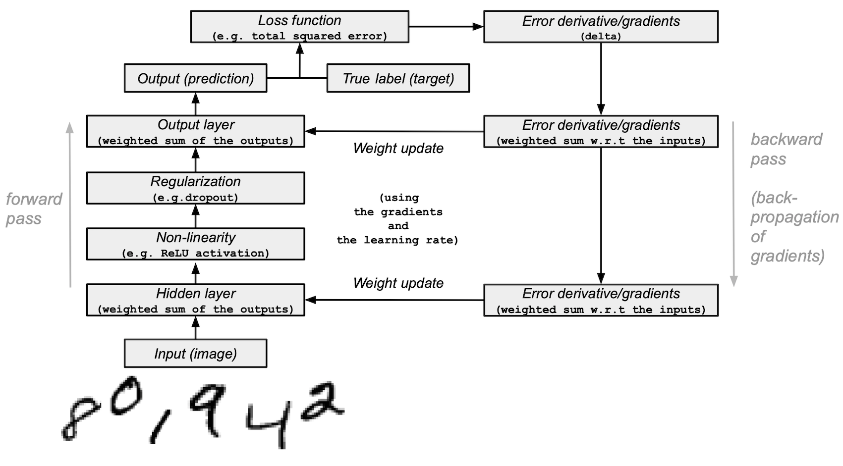
您将在模型中使用 1 个隐藏层来向前传递输入(前向传播)并将损失函数的梯度/误差导数向后传播(反向传播)。这些是输入层、隐藏层和输出层。
在隐藏层(中间层)和输出层(最后一层)中,神经网络模型将计算输入的加权和。为了计算这个过程,您将使用 NumPy 的矩阵乘法函数(“点乘”或 `np.dot(layer, weights)`)。
注意:为简单起见,在此示例中省略了偏置项(没有 `np.dot(layer, weights) + bias`)。
权重:这些是重要的可调参数,神经网络通过前向和后向传播数据来微调它们。它们通过称为 梯度下降 的过程进行优化。在模型训练开始之前,权重会使用 NumPy 的
Generator.random()进行随机初始化。最优权重应在训练集和测试集上产生最高的预测准确率和最低的误差。
激活函数:深度学习模型能够确定输入和输出之间的非线性关系,这些非线性函数通常应用于每个层的输出。
您将使用修正线性单元(ReLU)应用于隐藏层的输出(例如,`relu(np.dot(layer, weights))`)。
在本例中,您将使用一种称为 dropout 的方法——稀释——该方法会随机将层中的一些特征设置为 0。您将使用 NumPy 的
Generator.integers()方法定义它,并将其应用于网络的隐藏层。损失函数:该计算通过比较图像标签(真实值)与最后一层输出中的预测值来确定预测的质量。
为简单起见,您将使用基本的总平方误差,使用 NumPy 的 `np.sum()` 函数(例如,`np.sum((final_layer_output - image_labels) ** 2)`)。
准确率:该指标衡量网络在未见过的数据上进行预测的能力的准确性。
模型架构和训练摘要
以下是神经网络模型架构和训练过程的摘要:
输入层:
它是网络的输入——从 `training_images` 加载到 `layer_0` 的预处理数据。
隐藏层(中间层):
layer_1接收前一层的输出,并使用 NumPy 的 `np.dot()` 执行输入与权重(`weights_1`)的矩阵乘法。然后,该输出通过 ReLU 激活函数实现非线性,然后应用 dropout 以帮助防止过拟合。
输出层(最后一层):
layer_2接收 `layer_1` 的输出,并使用 `weights_2` 重复相同的“点乘”过程。最终输出为每个 0-9 数字标签返回 10 个分数。网络模型以一个大小为 10 的层结束——一个 10 维向量。
前向传播、反向传播、训练循环:
在模型训练开始时,您的网络会随机初始化权重,并将输入数据通过隐藏层和输出层向前馈送。这个过程是前向传播。
然后,网络将“信号”从损失函数反向传播通过隐藏层,并借助学习率参数(稍后将详细介绍)调整权重。
注意:更技术地说,您将
通过比较图像的真实标签(真实值)和模型的预测值来测量误差。
对损失函数进行微分。
摄取相对于输出的梯度,并通过层将它们相对于输入反向传播。
由于网络包含张量运算和权重矩阵,反向传播使用链式法则。
随着神经网络训练的每一次迭代(epoch),这种前向和后向传播的循环都会调整权重,这会反映在准确率和误差指标上。在训练模型时,您的目标是在模型学习的训练数据以及您评估模型的测试数据上最小化误差和最大化准确率。
编写模型并开始训练和测试它
在涵盖了主要的深度学习概念和神经网络架构之后,让我们来编写代码。
1. 我们将首先创建一个新的随机数生成器,提供一个种子以确保结果的可复现性。
seed = 884736743
rng = np.random.default_rng(seed)
2. 对于隐藏层,定义用于前向传播的 ReLU 激活函数以及在反向传播期间将使用的 ReLU 的导数。
# Define ReLU that returns the input if it's positive and 0 otherwise.
def relu(x):
    return (x >= 0) * x


# Set up a derivative of the ReLU function that returns 1 for a positive input
# and 0 otherwise.
def relu2deriv(output):
    return output >= 0
3. 设置一些 超参数 的默认值,例如:
学习率:`learning_rate` — 有助于限制权重更新的幅度,以防止它们过度修正。
Epoch(迭代次数):`epochs` — 数据通过网络的完整前向和后向传播的次数。此参数可能对结果产生积极或消极影响。迭代次数越多,学习过程可能需要的时间越长。因为这是一项计算密集型任务,我们选择了非常少的 epoch(20)。为了获得有意义的结果,您应该选择一个更大的数字。
网络中隐藏层(中间层)的大小:`hidden_size` — 隐藏层大小的不同会影响训练和测试期间的结果。
输入大小:`pixels_per_image` — 您已确定图像输入是 784(28x28)像素。
标签数量:`num_labels` — 指示输出层中预测 10 个(0 到 9)手写数字标签的输出数量。
learning_rate = 0.005
epochs = 20
hidden_size = 100
pixels_per_image = 784
num_labels = 10
4. 使用随机值初始化将在隐藏层和输出层中使用的权重向量。
weights_1 = 0.2 * rng.random((pixels_per_image, hidden_size)) - 0.1
weights_2 = 0.2 * rng.random((hidden_size, num_labels)) - 0.1
5. 设置神经网络的学习实验,包含一个训练循环并开始训练过程。请注意,在每个 epoch,模型都会根据测试集进行评估,以跟踪其在训练 epochs 中的性能。
开始训练过程
# To store training and test set losses and accurate predictions
# for visualization.
store_training_loss = []
store_training_accurate_pred = []
store_test_loss = []
store_test_accurate_pred = []

# This is a training loop.
# Run the learning experiment for a defined number of epochs (iterations).
for j in range(epochs):

    #################
    # Training step #
    #################

    # Set the initial loss/error and the number of accurate predictions to zero.
    training_loss = 0.0
    training_accurate_predictions = 0

    # For all images in the training set, perform a forward pass
    # and backpropagation and adjust the weights accordingly.
    for i in range(len(training_images)):
        # Forward propagation/forward pass:
        # 1. The input layer:
        #    Initialize the training image data as inputs.
        layer_0 = training_images[i]
        # 2. The hidden layer:
        #    Take in the training image data into the middle layer by
        #    matrix-multiplying it by randomly initialized weights.
        layer_1 = np.dot(layer_0, weights_1)
        # 3. Pass the hidden layer's output through the ReLU activation function.
        layer_1 = relu(layer_1)
        # 4. Define the dropout function for regularization.
        dropout_mask = rng.integers(low=0, high=2, size=layer_1.shape)
        # 5. Apply dropout to the hidden layer's output.
        layer_1 *= dropout_mask * 2
        # 6. The output layer:
        #    Ingest the output of the middle layer into the the final layer
        #    by matrix-multiplying it by randomly initialized weights.
        #    Produce a 10-dimension vector with 10 scores.
        layer_2 = np.dot(layer_1, weights_2)

        # Backpropagation/backward pass:
        # 1. Measure the training error (loss function) between the actual
        #    image labels (the truth) and the prediction by the model.
        training_loss += np.sum((training_labels[i] - layer_2) ** 2)
        # 2. Increment the accurate prediction count.
        training_accurate_predictions += int(
            np.argmax(layer_2) == np.argmax(training_labels[i])
        )
        # 3. Differentiate the loss function/error.
        layer_2_delta = training_labels[i] - layer_2
        # 4. Propagate the gradients of the loss function back through the hidden layer.
        layer_1_delta = np.dot(weights_2, layer_2_delta) * relu2deriv(layer_1)
        # 5. Apply the dropout to the gradients.
        layer_1_delta *= dropout_mask
        # 6. Update the weights for the middle and input layers
        #    by multiplying them by the learning rate and the gradients.
        weights_1 += learning_rate * np.outer(layer_0, layer_1_delta)
        weights_2 += learning_rate * np.outer(layer_1, layer_2_delta)

    # Store training set losses and accurate predictions.
    store_training_loss.append(training_loss)
    store_training_accurate_pred.append(training_accurate_predictions)

    ###################
    # Evaluation step #
    ###################

    # Evaluate model performance on the test set at each epoch.

    # Unlike the training step, the weights are not modified for each image
    # (or batch). Therefore the model can be applied to the test images in a
    # vectorized manner, eliminating the need to loop over each image
    # individually:

    results = relu(test_images @ weights_1) @ weights_2

    # Measure the error between the actual label (truth) and prediction values.
    test_loss = np.sum((test_labels - results) ** 2)

    # Measure prediction accuracy on test set
    test_accurate_predictions = np.sum(
        np.argmax(results, axis=1) == np.argmax(test_labels, axis=1)
    )

    # Store test set losses and accurate predictions.
    store_test_loss.append(test_loss)
    store_test_accurate_pred.append(test_accurate_predictions)

    # Summarize error and accuracy metrics at each epoch
    print(
        (
            f"Epoch: {j}\n"
            f"  Training set error: {training_loss / len(training_images):.3f}\n"
            f"  Training set accuracy: {training_accurate_predictions / len(training_images)}\n"
            f"  Test set error: {test_loss / len(test_images):.3f}\n"
            f"  Test set accuracy: {test_accurate_predictions / len(test_images)}"
        )
    )
Epoch: 0
Training set error: 0.898
Training set accuracy: 0.397
Test set error: 0.680
Test set accuracy: 0.582
Epoch: 1
  Training set error: 0.656
  Training set accuracy: 0.633
  Test set error: 0.607
  Test set accuracy: 0.641
Epoch: 2
  Training set error: 0.592
  Training set accuracy: 0.68
  Test set error: 0.569
  Test set accuracy: 0.679
Epoch: 3
  Training set error: 0.556
  Training set accuracy: 0.7
  Test set error: 0.541
  Test set accuracy: 0.708
Epoch: 4
  Training set error: 0.534
  Training set accuracy: 0.732
  Test set error: 0.526
  Test set accuracy: 0.729
Epoch: 5
  Training set error: 0.515
  Training set accuracy: 0.715
  Test set error: 0.500
  Test set accuracy: 0.739
Epoch: 6
  Training set error: 0.495
  Training set accuracy: 0.748
  Test set error: 0.487
  Test set accuracy: 0.753
Epoch: 7
  Training set error: 0.483
  Training set accuracy: 0.769
  Test set error: 0.486
  Test set accuracy: 0.747
Epoch: 8
  Training set error: 0.473
  Training set accuracy: 0.776
  Test set error: 0.473
  Test set accuracy: 0.752
Epoch: 9
  Training set error: 0.460
  Training set accuracy: 0.788
  Test set error: 0.462
  Test set accuracy: 0.762
Epoch: 10
  Training set error: 0.465
  Training set accuracy: 0.769
  Test set error: 0.462
  Test set accuracy: 0.767
Epoch: 11
  Training set error: 0.443
  Training set accuracy: 0.801
  Test set error: 0.456
  Test set accuracy: 0.775
Epoch: 12
  Training set error: 0.448
  Training set accuracy: 0.795
  Test set error: 0.455
  Test set accuracy: 0.772
Epoch: 13
  Training set error: 0.438
  Training set accuracy: 0.787
  Test set error: 0.453
  Test set accuracy: 0.778
Epoch: 14
  Training set error: 0.446
  Training set accuracy: 0.791
  Test set error: 0.450
  Test set accuracy: 0.779
Epoch: 15
  Training set error: 0.441
  Training set accuracy: 0.788
  Test set error: 0.452
  Test set accuracy: 0.772
Epoch: 16
  Training set error: 0.437
  Training set accuracy: 0.786
  Test set error: 0.453
  Test set accuracy: 0.772
Epoch: 17
  Training set error: 0.436
  Training set accuracy: 0.794
  Test set error: 0.449
  Test set accuracy: 0.778
Epoch: 18
  Training set error: 0.433
  Training set accuracy: 0.801
  Test set error: 0.450
  Test set accuracy: 0.774
Epoch: 19
  Training set error: 0.429
  Training set accuracy: 0.785
  Test set error: 0.436
  Test set accuracy: 0.784
训练过程可能需要数分钟,具体取决于许多因素,例如您运行实验的机器的处理能力以及 epoch 的数量。为了减少等待时间,您可以将 epoch(迭代次数)变量从 100 更改为一个较小的数字,重置运行时(这将重置权重),然后再次运行 notebook 单元格。
执行完上面的单元格后,您可以可视化此训练过程中训练和测试集的误差和准确率。
epoch_range = np.arange(epochs) + 1  # Starting from 1

# The training set metrics.
training_metrics = {
    "accuracy": np.asarray(store_training_accurate_pred) / len(training_images),
    "error": np.asarray(store_training_loss) / len(training_images),
}

# The test set metrics.
test_metrics = {
    "accuracy": np.asarray(store_test_accurate_pred) / len(test_images),
    "error": np.asarray(store_test_loss) / len(test_images),
}

# Display the plots.
fig, axes = plt.subplots(nrows=1, ncols=2, figsize=(15, 5))
for ax, metrics, title in zip(
    axes, (training_metrics, test_metrics), ("Training set", "Test set")
):
    # Plot the metrics
    for metric, values in metrics.items():
        ax.plot(epoch_range, values, label=metric.capitalize())
    ax.set_title(title)
    ax.set_xlabel("Epochs")
    ax.legend()
plt.show()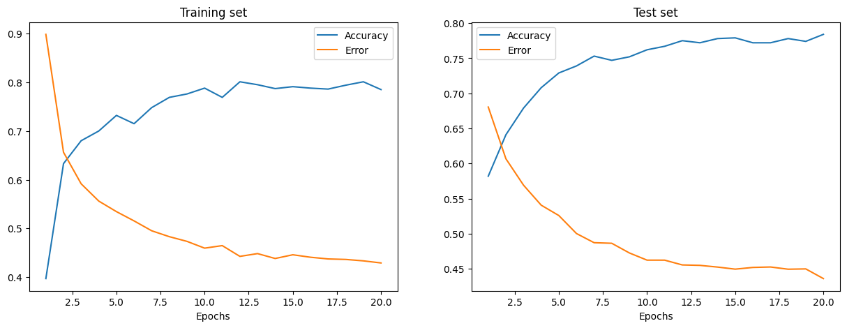
训练和测试误差分别显示在左侧和右侧的图中。随着 Epochs 数量的增加,总误差减小,准确率提高。
您的模型在训练和测试期间达到的准确率可能还可以,但误差率也可能相当高。
为了在训练和测试期间减少误差,您可以考虑将简单的损失函数更改为,例如,分类 交叉熵。其他可能的解决方案将在下面讨论。
下一步
您已经学会了如何仅使用 NumPy 从头开始构建和训练一个简单的前馈神经网络,以对 MNIST 手写数字进行分类。
为了进一步增强和优化您的神经网络模型,您可以考虑以下一项或多项措施:
将训练样本量从 1,000 增加到更大的数量(最多 60,000)。
使用小批量并降低学习率。
通过引入更多隐藏层来更改架构,使网络更深。
引入卷积层:用卷积神经网络架构替换前馈网络。
引入验证集以无偏地评估模型拟合情况。
应用批标准化以实现更快、更稳定的训练。
调整其他参数,例如学习率和隐藏层大小。
从头开始使用 NumPy 构建神经网络是深入了解 NumPy 和深度学习的好方法。然而,对于实际应用,您应该使用专门的框架——例如 PyTorch、JAX、TensorFlow 或 MXNet——这些框架提供类似 NumPy 的 API,具有内置的自动微分和 GPU 支持,并且专为高性能数值计算和机器学习而设计。
最后,在开发机器学习模型时,您应该考虑潜在的道德问题,并采取措施避免或缓解这些问题。
使用模型卡片记录已训练的模型——请参阅 Margaret Mitchell 等人的 模型卡片用于模型报告论文。
使用数据集数据表记录数据集——请参阅 Timnit Gebru 等人的 数据集数据表论文。
更多资源,请参阅 Rachel Thomas 的这篇博文和 Radical AI 播客。
(感谢 hsjeong5 展示了如何在不使用外部库的情况下下载 MNIST。)
- Mitchell, M., Wu, S., Zaldivar, A., Barnes, P., Vasserman, L., Hutchinson, B., Spitzer, E., Raji, I. D., & Gebru, T. (2019). Model Cards for Model Reporting. Proceedings of the Conference on Fairness, Accountability, and Transparency, 220–229. 10.1145/3287560.3287596